


Cyber-Physical Systems are cyber systems controlling physical entities, these entities being, for instance, mechanical or biological. Their development involves different engineering disciplines that use different models, written in languages with different semantics. These heterogeneous models are participating in the dynamic of the system and a coupled simulation of these models can be used to understand the system behavior.
The Functional Mock-up Interface is a standard for co-simulation that provides a time-driven API to communicate between the solvers of different models. At runtime, data can then be exchanged between the different models to represent the interaction between the models.In this webpage, we shown the limitations there exist in FMI when used with cyber models, where event and discontinuity in variable are natural phenomenon. This limitations introduce bad performance and inaccuracy (both temporal and functional). We proposed backward compatible extensions to the FMI API in order to allow efficient and correct use of cyber models during co-simulation with FMI. We implemented these extensions and we shown that our approach globally provide better performances and very good accuracy. For the experiments we obtained cyber FMUs by developing an export of VHDL models into FMU and we reused the JModelica FMU compiler for physical models.
Overview
This companion web page presents some artifacts and results mentioned in the paper submitted to RAPIDO 2018.
It provides an overview of the steps to launch the experiments using the FMI extensions proposed and their results. The user will require downloading the source code and follow the steps describe in part 1 and 2.
Currently, the tests run on Ubuntu 16.04 x86_64.
Part 1: Download and compile source code
First, download the source code (.tar.gz) from here.
To compile the source code, all these dependencies must be satisfied:
- g++
- CMake
- gnuplot
- libgfortran-4.8-dev
- libexpat1-dev
- libxml2-dev
Then, in the terminal:
$ mkdir build
$ cd build
$ cmake ..
$ make
Each test case has two implementations: one using the proposed APIs and one using the current API (v2.0).
At the end of each simulation, the simulator creates two files for each FMU. The first file is a .csv, it contains a trace of the simulation, the second one is a .png image created from the trace inside the .csv. All the benchmarks were executed with the benchmark flag, without any write on disk, all the logs disable and internal tracing disable.
Part 2: Examples and Experimental results
Example 1: Wheel encoder driver
Outline:
1. Implementation
2. FMU wrapper
3. FMU model
4. Results
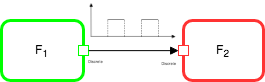
The first example is a system composed of a wheel encoder driver FMU and a speed computation FMU. It is used to describe the fmi2SimulateUntilDiscontinuity API and run benchmarks on it.
To compile and run it, run in the terminal:
$ make sim_wheel_encoder_fidel
$ cd bin
$ ./sim_wheel_encoder_fidel
Implementation
Inside the model, the fmi2SimulateUntilDiscontinuity API is implemented as described in the following sections.
FMU wrapper
The wrapper it’s called fmuInterface and it’s used to communicate between the MA and the internal model of the FMU. It exposes the fmi2SimulateUntilDiscontinuity function to execute the model.
    fmi2Status fmi2SimulateUntilDiscontinuity(fmi2Component c,
                        fmi2Real currentCommunicationPoint, fmi2Port* ports,
                        size_t nPorts, fmi2Real* nextEventTime)
    {
        ModelInstance* comp = (ModelInstance*)c;
        generator* g = (generator*) comp->model;

        // Update global time (current communiaction point)
        comp->globalTime = currentCommunicationPoint;
        // Update ports under eventMode
        g->ports = ports;
        g->nPorts = nPorts;
        // Run the simulation until an event occur
        simulate_and_wait(comp, fmi2False);
        *nextEventTime = comp->time;
        return fmi2OK;
    }
It sets the global time inside the model and the watching variables if there is a write operation on one of them, the model returns. Then, it calls simulate_and_wait to start the simulation or to resume the model. We implemented the pause/resume mechanism using mutexes.
fmi2SimulateUntilDiscontinuity calls this function to execute the model until a change occurs.
void simulate_and_wait(fmi2Component c, fmi2Boolean oneCycle)
{
  ModelInstance* comp = (ModelInstance*) c;
  generator* g= (generator*) comp->model;
  comp->justOneCycle = oneCycle;
  if (oneCycle)
  {
    while(!comp->cycleCompleted)
    {
      pthread_mutex_unlock(&g->m1);
      pthread_mutex_lock(&g->m2);
    }
   }
   else
   {
     pthread_mutex_unlock(&g->m1);
     pthread_mutex_lock(&g->m2);
    }
  // Save the current pending variable
  set_pending_variable(comp);
}
simulate_and_wait unlocks the model thread and waits for an unlock event.
During the initialization phase, the main thread forks another thread and load on it the function simulateUntil. This function represents the thread model; the model execution is running on it. This function calls simulate() to run the model for 1 cycle. If something changes during the execution, this thread is locked from inside the model. Otherwise, the function returns and continues until a change occurs.
void* simulateUntil(void* data)
{
  ModelInstance* comp = (ModelInstance*) data;
  counterwave* g= (counterwave*) comp->model;
  counterwave::counterwave_iostruct* io_exchange = (counterwave::counterwave_iostruct*) comp->iostruct;
  comp->threadStarted = fmi2True;
  pthread_mutex_lock(&g->m1);
  while(comp->threadStarted)
  {
    // Step is not completed
    comp->cycleCompleted = fmi2False;
    // Run the real simulation
    g->simulate(io_exchange, comp->cycle_number);
    // Internal clock
    io_exchange->clock = !io_exchange->clock;
    // Tag this step as Completed
    comp->cycleCompleted = fmi2True;
    // One cycle simulation, until we reach the time requested
    if (comp->justOneCycle && ( comp->time > comp->globalTime))
    {
      // Reset to false just one cycle
      comp->justOneCycle = fmi2False;
      // Unlock counterwave_simulate_and_wait
      pthread_mutex_unlock(&g->m2);
      pthread_mutex_lock(&g->m1);
    }
  }
pthread_exit(NULL);
}
FMU model
The function postWriteOutputPort is called every time the model writes on an output variable. Inside this function, there is a check if the variable is a monitored variable. If it is true, then the model unlocks the main thread containing the wrapper and waits until the simulator resumes it. When this method returns, the model continues its execution.
void generator::postWriteOutputPort(char* nameOfTheVariable)
{
    for(int i = 0; i < nPorts; ++i)
    {
        if (ports[i].type == Boolean && ports[i].vref == 0)
        {
            isWriting = true;
            variableUnderRead = nameOfTheVariable;
            pthread_mutex_unlock(&m2);
            // Wait until the main thread unlock this thread
            pthread_mutex_lock(&m1);
            isWriting = false;
        }
    }
}
Results
The following figure shows the results obtained simulating the example using the new APIs. The golden model traces the simulation results expected, the green dots are the simulation results using the new approach. As we show in the paper, the coordinator pauses the simulation and retrieves the updated value. 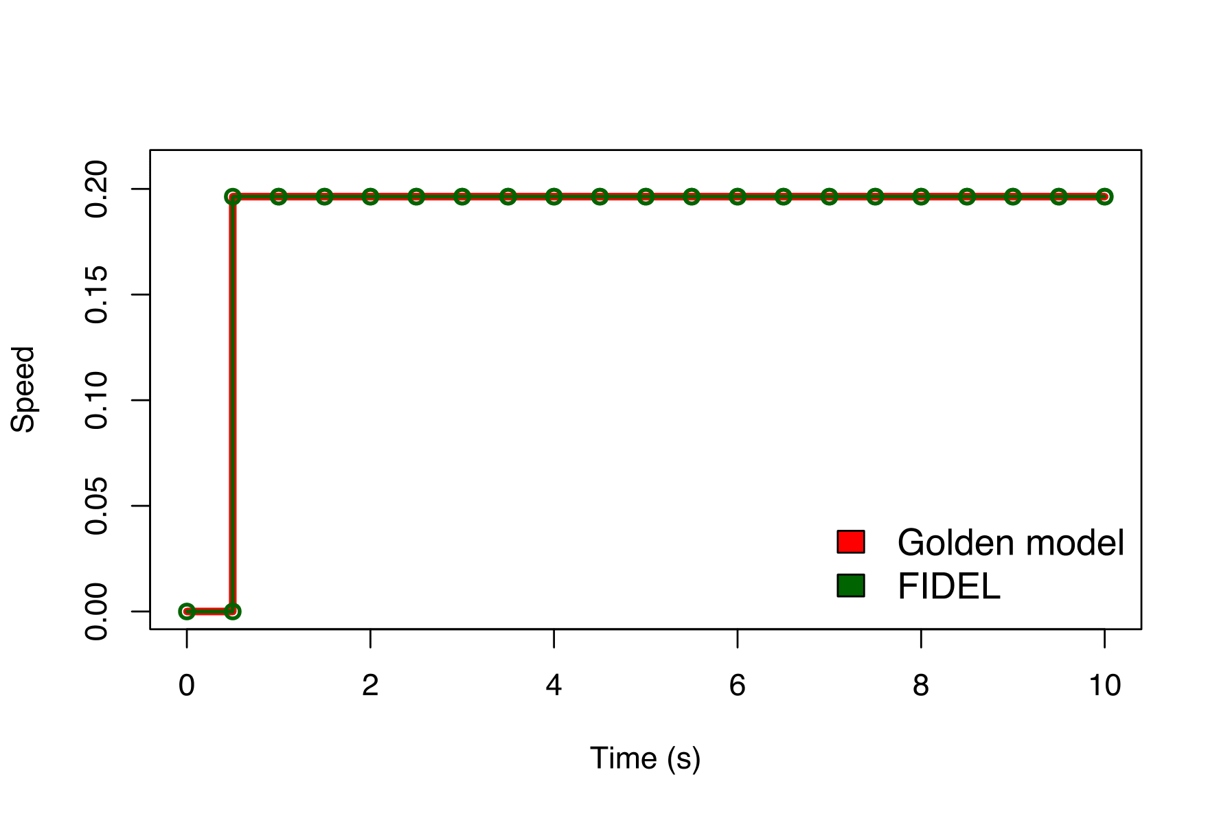
Example 2: Sensor and environment
In this example, we want to highlight the precision and performance gain in case there are input variables.
Sections:
Implementation
Results
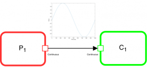
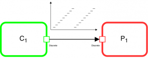
The figure shows how the two FMUs are linked together. The graph shows the signal from the environment FMU to the sensor FMU.
To build and execute the example, launch these command:
$ make sim_sensor_env_fidel
$ cd bin
$ ./sim_sensor_env_fidel
Implementation
The sensor implementation is similar to the previous one, except for two specific functions.
The first one is the fmi2SimulateUntilRead implementation.
fmi2Status fmi2SimulateUntilRead(fmi2Component c, fmi2Real currentCommunicationPoint,
    fmi2Port* ports, size_t nPorts, fmi2Real* nextEventTime)
{
    ModelInstance* comp = (ModelInstance*)c;
    sensor* g = (sensor*) comp->model;
    // Update global time (current communiaction point)
    comp->globalTime = currentCommunicationPoint;
    // Update ports under eventMode
    g->ports = ports;
    g->nPorts = nPorts;
    // Run the simulation until an change occurs
    sensor_simulate_and_wait(comp, fmi2False);
    *nextEventTime = comp->time;
    return fmi2OK;
}
In the following C++ code snippet is described how the “pause” mechanism is implemented. The u variable represents an input port of the model. Just before its value is assigned to another variable, the model calls the preReadInputPort function to pause the model and resume the main thread. When the main thread wants to resume the simulation, the preReadInputPort returns and the simulation continues (in this case, the variable u assigns its value to y)
...
if ( sensor_pack::st_1 == next_status)
{
 preReadInputPort("u");
 hif_a2t_data.y = hif_a2t_data.u;
 counter_new = 0L;
}
...
The preReadInputPort is similar to the postWriteOutputPort except it handles the read operations. It sets the operation as a reading operation and then, if the variable is inside the watching variables, it unlocks the main thread and waits until the reading value is ready.
void sensor::preReadInputPort(char* nameOfTheVariable)
{
  isReading = true;
  for(int i = 0; i < nPorts; ++i)
  {
    if (ports[i].type == Real && ports[i].vref == 0)
    {
      variableUnderRead = nameOfTheVariable;
      pthread_mutex_unlock(&m2);
      pthread_mutex_lock(&m1);
    }
  }
isReading = false;
}
Results
We run tests to investigate the impact of the proposed API and the limitations of the current one. All tests run the simulation for 10 seconds (simulated time). The sensor senses the environment every 50ms.
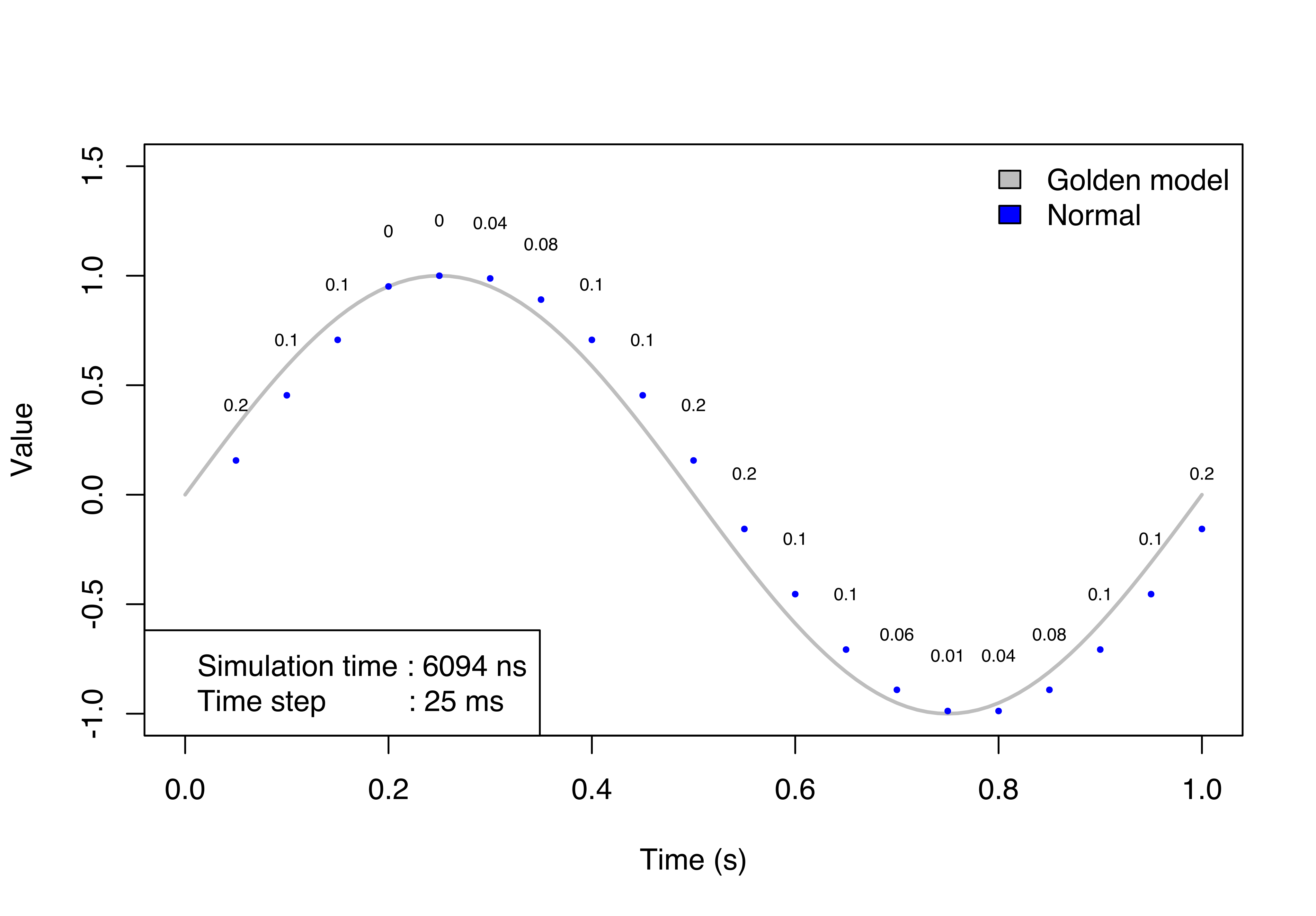
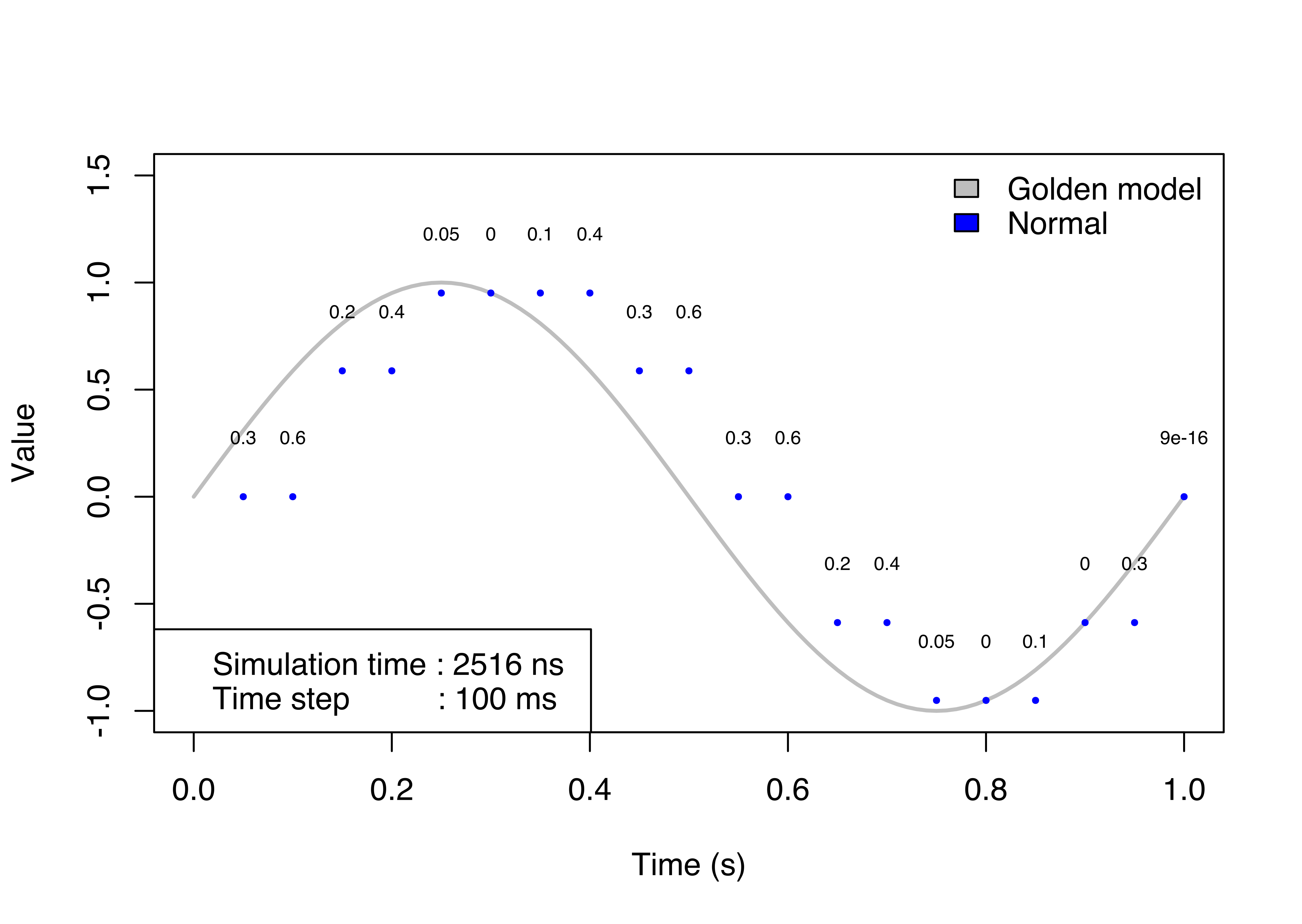
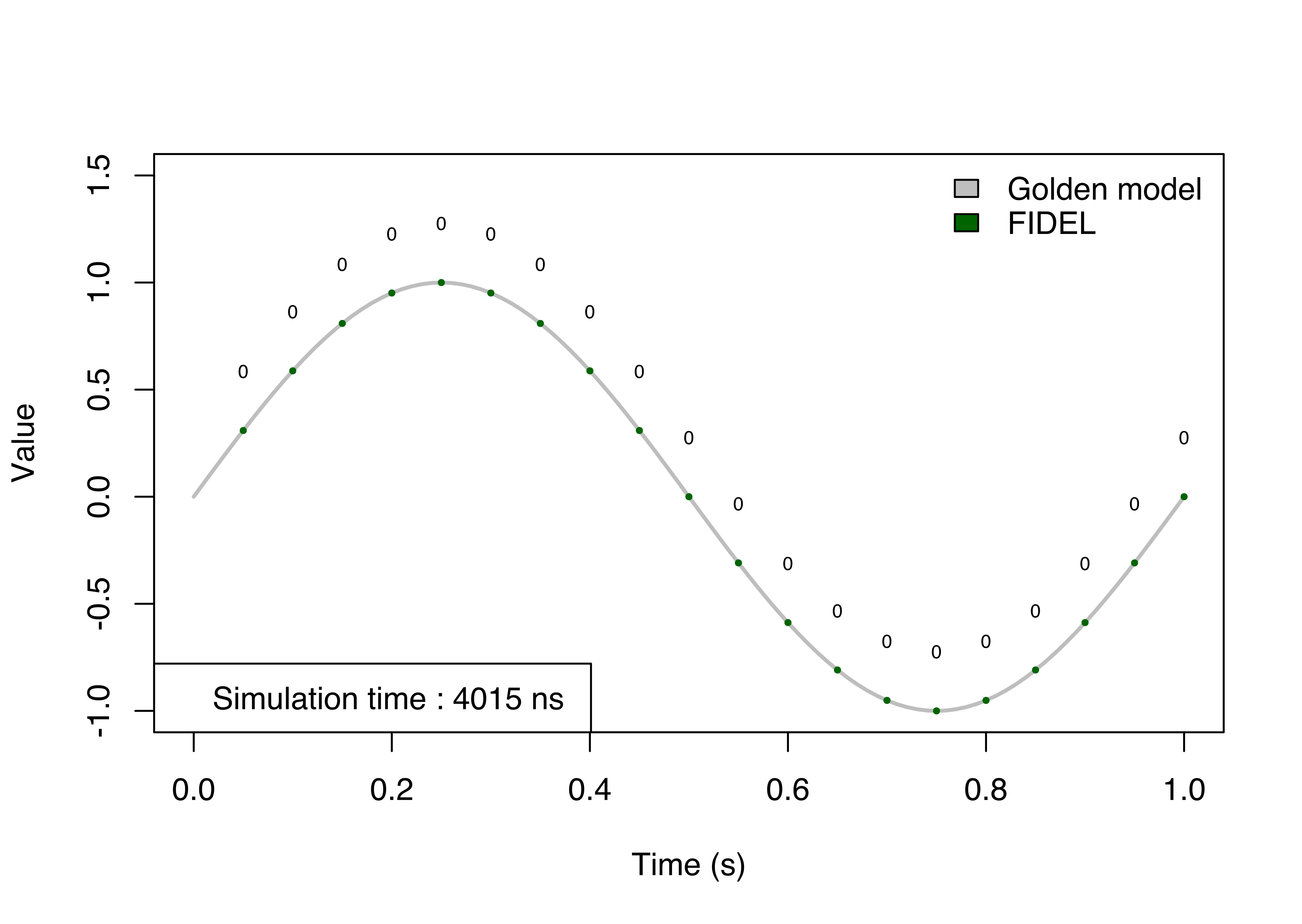
The number above the curve is the error between the golden model value and the value reads by the model. It represents the absolute vertical error between the two values at the same instant. The different value generates a shifted curve along the time axis. It doesn’t mean values are delayed but it is an error during the read operation because the model reads an outdated value.
In the first image, the step size is half the value of the internal sample rate of the sensor. The simulation is quite accurate, but it has a small error due to the time-driven approach. The error is maximum the sinus of the step size because if the sensor reads just before the end of the step size, it gets the value for the previous time instant. If the performance is more important than the accuracy, the step size can be increased but the simulation will be completely wrong. In the last picture, there are the results for the FIDEL approach. It has no error
Example 3: Modulo counter
In this example, we want to improve performances limiting the communication points at the minimum required. The modulo counter counts until it reaches a threshold and then starts the count again. The idea behind this API is to limit the communication points using constraints. If a second FMU needs a particular value to activate, it exposes a constraint to limit the communication only when the first FMU reaches this constraint.
Sections:
Implementation
Best normal
Results
$ make sim_modulo_counter_fidel_conditional
$ cd bin
$ ./sim_modulo_counter_fidel_conditional
Implementation
Inside the model, this mechanism is implemented as follows:
void counterwave::postWriteOutputPort(char* nameOfTheVariable)
{
  // Check if variable is inside ports array
  for(int i = 0; i < nPorts; ++i)
  {
    if (ports[i].type == Integer && ports[i].vref == 0)
    {
      fmi2Port p;
      p.type = Integer;
      p.vref = 0;
      p.ivalue = hif_a2t_data.dataout;
      if (ports[i].callbackCondition != NULL)
      {
        if (ports[i].callbackCondition(p))
        {
          isWriting = true;
          variableUnderRead = nameOfTheVariable;
          pthread_mutex_unlock(&m2);
          pthread_mutex_lock(&m1);
          isWriting = false;
        }
      }
      else
      {
        isWriting = true;
        variableUnderRead = nameOfTheVariable;
        pthread_mutex_unlock(&m2);
        pthread_mutex_lock(&m1);
        isWriting = false;
      }
    }
  }
}
It checks if the variable, passed as the parameter, is in the watching list. If it is present then it checks the condition calling the callbackCondition() function on the port. This function is a callback registered by the MA during the initialization phase. When the condition is true, the function returns true and the model pauses itself, the mechanism to pause it, it’s the same as the previous examples. The callback is provided by the FMU that is linked on this FMU and requires a specific value to activate itself.
In this case, the function is fCheckInput(fmi2Port p) and it’s implemented as follows:
fmi2Boolean fCheckInput(fmi2Port p)
{
  static int p_old = 0;
  int res = (( p_old >= 50 && p.ivalue < 50) || (p_old <= 50 && p.ivalue > 50));
  p_old = p.ivalue;
  return res;
}
For a better reading, the function is written inside the MA but it can be located also inside the FMU target. The FMU target is the model that reads the output variable to execute. In this case, the function postWriteOutputPort() has to call the callback registered in the other FMU.
It checks if the variable, represented as a fmi2Port, meets the constraints and returns true or false. If it returns true, the value is usable and it can be used by another FMU as a valid value. It means the FMU has to pause itself and the MA has to trigger the FMU that requires that value.
Best Normal
The Best Normal is a new type of Master Algorithm to emulate the mechanism of the new API using the current API.
It uses the same idea it’s behind the conditional API: it runs a single FMU until it reaches a particular value on one of its output ports by using the existing fmi2DoStep API. However, the run of the other FMU is done only when the condition of the previous value is true. In this case, it limits the number of communication point but there is an error as in the normal approach due to the time-driven simulation (see above).
Results
The following table shows benchmarks of the example, using the Normal, Best Normal and FIDEL API. The results show how the FIDEL approach can improve the performance decreasing the number of communication points. In the best normal test, the first number of communication is the number of CP with the Counter time FMU and the second the number of CPs with the Slope FMU. Although in this approach, the counter FMU communicates with the MA as many times as in the normal approach without sharing any data with the slope FMU, it reduces the number of communication points with the slope FMU.
In fact, the slope FMU decreases its simulation time but the counter FMU, except in the first case, has the same simulation time.
The last result shows the performances of the FIDEL approach using the minimum of the CPs required, in agreement with the given constraints. There is the same amount of CPs as in the best normal but, in this case, the counter FMU communicates less with the MA and it stops when it reaches one of the constraints.
If we want the same performance gain using the normal approach, we can increase the step size but, as a drawback, we have a less accurate simulation.
| Normal | Best normal | FIDEL conditional | |||||||
|---|---|---|---|---|---|---|---|---|---|
| Step size (ms) | CPs | Counter time (ns) | Slope time (ns) | CPs | Counter time (ns) | Slope time (ns) | CPs | Counter time (ns) | Slope time (ns) |
| 1 | 10000 | 6922 | 72769 | 10000/40 | 3367 | 542 | 40 | 1227 | 383 |
| 5 | 2000 | 2201 | 13474 | 2000/40 | 2122 | 584 | |||
| 50 | 200 | 1199 | 1274 | 200/40 | 988 | 304 | |||