
Here are test cases of simulated reflectors with blender and a comparison between solvers.
-
PIR0
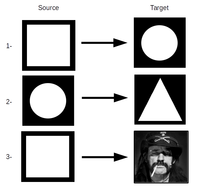
Three test cases for PIR0. 1- Uniform square to uniform disc. 2- Uniform disc to uniform triangle. 3- Uniform square to Lemmy Kilmister portrait.
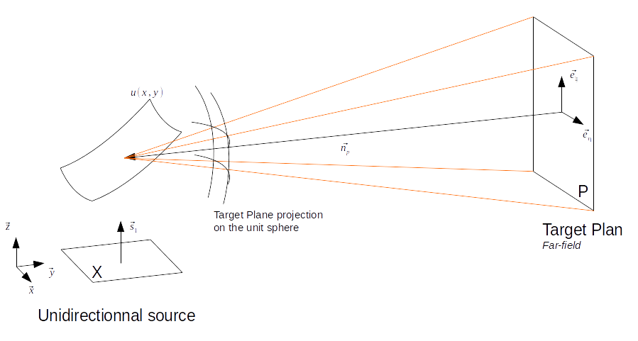
Keeping the notations of the PIR0 configuration schematic, the geometrical configuration is as follow:
\(\displaystyle \vec{s_1} = \begin{pmatrix} 1\\0\\0 \end{pmatrix}, \ \ \ \vec{e_{\eta}} = \begin{pmatrix} 0\\-1\\0 \end{pmatrix}, \ \ \ \vec{e_{\xi}} = \begin{pmatrix} 0\\0\\1 \end{pmatrix}, \ \ \ \vec{n_{p}} = \begin{pmatrix} -5000\\0\\0 \end{pmatrix}\)
The source support is \(\displaystyle [-5, 5]\times[-5,5]\) and the target plan support is \(\displaystyle [-500, 500]\times[-500,500]\).
It is important to choose a large \(\displaystyle \| \vec{n_p}\|\) and a large target plan support compared to the source support to ensure correct far-field conditions, otherwise deformations will occur at the rendering step.
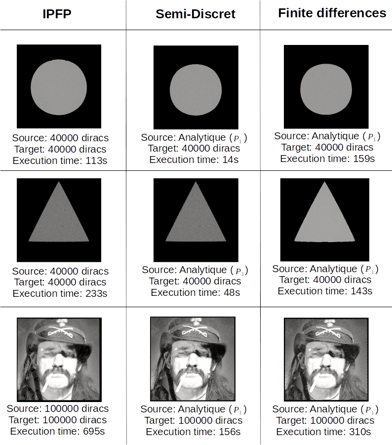
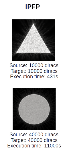
Results of the reflector simulation with Blender. First column is IPFP, second is Semi-Discrete and third is Finite differences. Below each picture are the source and target resolution and the execution time.
-
PIR1
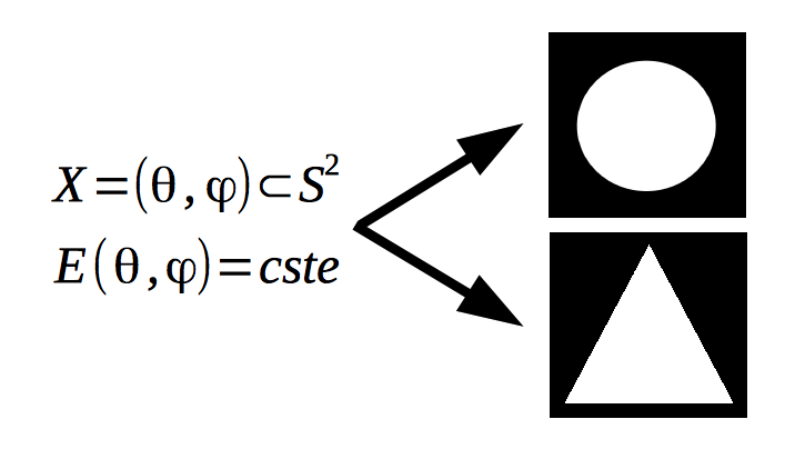
Two test case for PIR1. In both cases the source is an emission cone of uniform light.
The geometrical configuration in these cases is as follow:
\(\displaystyle \vec{s_1} = \begin{pmatrix} 1\\0\\0 \end{pmatrix}, \ \ \ \vec{e_{\eta}} = \begin{pmatrix} 0\\-1\\0 \end{pmatrix}, \ \ \ \vec{e_{\xi}} = \begin{pmatrix} 0\\0\\1 \end{pmatrix}, \ \ \ \vec{n_{p}} = \begin{pmatrix} -500\\0\\0 \end{pmatrix}\)
The source opening angle is \(\displaystyle \frac{\pi}{20}\) and the target plan support is \(\displaystyle [-50, 50]\times[-50,50]\).
Results of the PIR1 reflector simulation with Blender.
As describe in the Solver part of Numerical Methods, the optimized version of the IPFP algorithm is not available yet, explaining the very long execution time compared to PIR0.