


A test of ICA algorithms with instantaneous mixtures
This code is a standard test of ICA algorithms. An instantaneous mixture of J signals is generated where the mixing matrix is random. The mixture is separated by selected methods and the standard criterion Signal-to-Interference Ratio (SIR) is evaluated on each separated signal.
This test can be used to observe the dependence of the algorithms on various factors (the length of data, the number of signals, computational burden, reliability, etc.). An important factor is the character/model/origin of the signals. Here, we mix artificial and speech signals. The artificial signals obey the standard ICA models described in the chapter (nongaussian i.i.d., piecewise Gaussian i.i.d, and Gaussian weak stationary – autoregressive). It means that some of these signals need not be separable by a given method that utilizes only some signal diversities (nongaussianity, nonstationarity, non-whiteness).
Various ICA/BSS algorithms can be compared this way. We recommend trying methods (but not only) from the following links: MLSP-Lab, A.S.A.P., Petr Tichavsky, ICALAB toolbox, FastICA, LVA central
The code of the test is available here.
Separation of real-world recordings
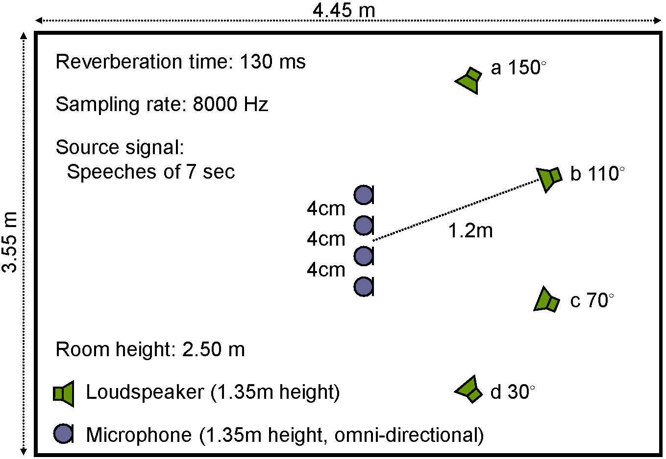
Here, the data of the example that is presented in the chapter are provided. The experimental setup is shown in the picture above. Four loudspeakers and microphones were located in a room where the distance of the loudspeakers from microphones was 1.2 m. Each loudspeaker was situated at different angle. Two male and two female utterances (dataset A and dataset B) were each played by the respective loudspeaker at a different angle. The spatial images (dataset A and dataset B) of the signals were recorded by the microphones. The mixed signals (dataset A and dataset B) are equal to the sum of the spatial images of the individually recorded sources.
Three setups were considered with two (a and b), three (a through c) and four (a through d) sources. The number of used microphones was the same as that of the sources in each setup. The mixtures were separated by three methods: FD-ICA with activity sequence (power ratio) clustering (dataset A and dataset B), FD-ICA with TDOA estimations (dataset A and dataset B), and FastIVA (dataset A and dataset B). The results are available for different lengths of the STFT (from 128 through 4096).
Separation of simulated convolutive audio mixtures
This code simulates acoustic mixtures of two, three or four speakers. Room impulse responses between the sources and microphones are generated by the image method implemented by Emmanuel Habets; please download the package from AudioLabs. The sources and the microphones can be placed at any point in the room; default locations are defined in the code.
The user can apply any BSS method to the artificial mixture. As a reference method, the time-domain T-ABCD algorithm is used; please download the T-ABCD package. T-ABCD can be used to estimate only short filters (10-80 taps) since its computational complexity rapidly grows with the length of filters. It is robust but it cannot handle long tails of the impulse responses (only direct path and early reflections) as the separating filters are short. The reader is encouraged to compare T-ABCD with the FD-ICA approaches described in the chapter.
The evaluation is done using the BSS_EVAL toolbox where there are four criteria: SDR, SIR, ISR and SAR. Please, download the package here a see the corresponding publication for the definition of the criteria.
Real-world convolutive audio mixtures
The graphical user interface of T-ABCD can be used to create stereo recordings. Users can conduct a real-world experiment with two microphones and two simultaneously speaking persons. We recommend that the speakers are about 1 m distant from the microphones (larger distance makes the mixture more difficult to separate) and do not perform any movements during recording. The mutual distance of microphones should be small (say about 10 cm) so that short separating filters can separate the recordings. Then, T-ABCD can be directly applied. The separation performance depends on many aspects such as on the angle between the speakers or their distance from microphones or on the reverberation time.
Hint: Check if your audio recording device is indeed stereo. Some low-cost sound cards do not support two-channel recordings and mix both channels (microphones) into a mono channel.
Theoretical exercises
- Define joint entropy of n random variables, and derive (13.12) using the definition of mutual information (13.11) and the definition of entropy (13.13).
- Show that the joint entropy of n random variables is constant under the orthogonal constraint (the random variables are uncorrelated and all have variance one).
- Show that the preprocessed signals defined by (13.29) are orthogonal and have unit variance.
- Consider two or more Gaussian piecewise stationary signals that are independent a have the same variance profiles (the same variance within each block of stationarity); the piecewise stationary model is introduced in Section 13.2.3.1. Show that the signals cannot be separated through the approximate joint diagonalization of their covariance matrices on blocks. Find an analogy for the model described in Section 13.2.3.2.