


Exercises:
Exercise 1: GCC-PHAT & Acoustic Maps
Given a speech signal of a static human source recorded in a real multi-channel acquisition set up, compute the GCC-PHAT focusing on:
- temporal evolution of the GCC-PHAT due to speech sparsity;
- behaviour of GCC-PHAT at different microphone pairs.
Using the computed GCC-PHAT, derive the corresponding GCF (SRP-PHAT) acoustic map.
The package include:
- audio signals;
- Matlab scripts with:
- functions to read and de-interlace audio files;
- a simple implementation of GCC-PHAT;
- microphone and source nominal positions;
- pseudo-code for GCF (SRP-PHAT) computation.
The figure on the left shows the layout of the experimental set up. The source is oriented downward. Note that the Matlab script is not optimized to allow an easier reading.
Exercise 2: Effect of microphone array geometry on source localization
For a near-field source, the TDOA equation is written in Chapter 3 of the book (Eq.3.8). A small error in the TDOA measurement is reflected on the source position s in a way that depends on the microphone and sensor geometry. By investigating the partial derivative of TDOA w.r.t. source position ∂τ/∂s, i.e. the Jacobian matrix J, we can quantify the expected behavior of the localization error with Gaussian noise in the TDOA estimate τ (zero mean, standard deviation σ).
Question 1: Derive the Jacobian matrix J. Hint: use vector form of TDOA equation,τii’= (||s–mi||-||s–mi’||)/c and differentiate it with respect to vector s, where mi and mi’ are the two microphone position of a single microphone pair.
Question 2: Take a look at the Matlab program code to reproduce the position error figures in Chapter 4. (You need to download an external Matlab tool called error_ellipse, that plots the error ellipse using a mean and covariance matrix).
Provided material: Matlab implementation for the error analysis: error visualization code
Note that only two microphone pairs are used. Consider the two following exercises:
- In the code, replace the current microphone setup with a circular microphone array of 8 elements and diameter 15 cm. Place a source at 2m distance from array center. How does the error ellipse look like?
- Intuitively, in such geometry estimating the 3D source position is difficult, while direction of arrival is easier to obtain. Does the resulting error ellipse support this or not?
Exercise 3: Tracking with particle filter
This exercise deals with tracking a moving source in a distributed microphone recording set up consisting of 7 triplet of microphones. Data are recorded in FBK labs and the ground truth trajectory was obtained using a multi-camera target tracking system. The speaker is silent twice during the recording. The figures below show the recording set up, the speaker trajectory and the audio file recorded at 1 channel of the acquisition network.
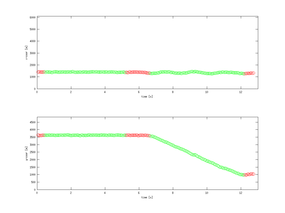
Source trajectory in the x- and y-coordinate
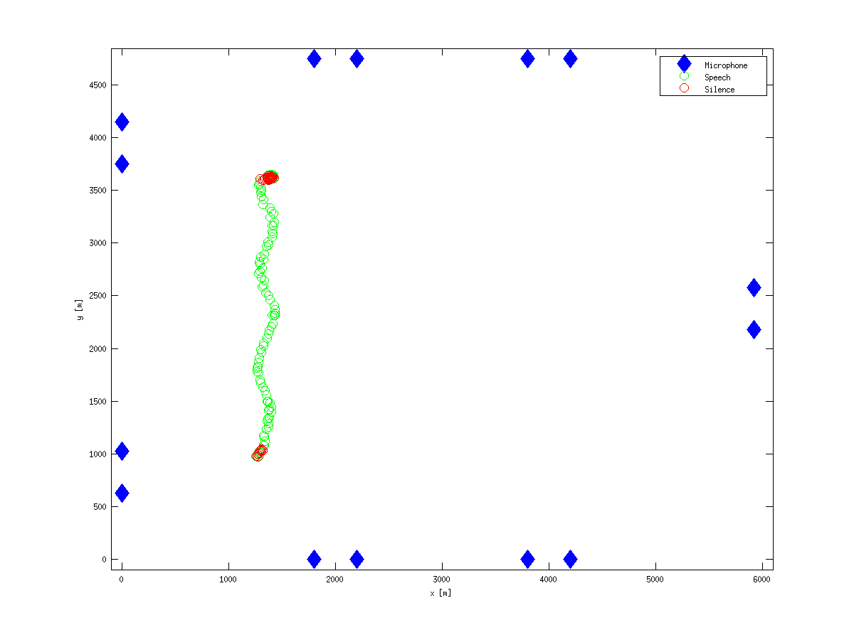
Position of the microphone triplets and speaker trajectory. Green dots indicate trajectory portions where the source was active, red segments correspond to silence.

Audio signal (channel 1)
The package includes:
- Audio files: raw 16 bit, 14 interlaced channels at 44.1 kHz.
- Reference trajectory=[time x y]n
- Matlab script to be completed with localization and tracking algorithms
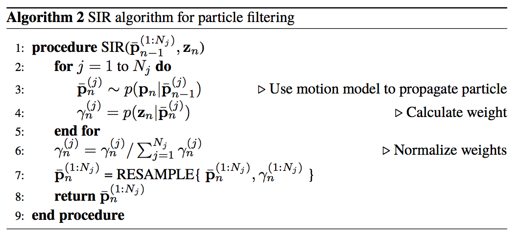
Question: Complete the script filling in the empty spaces and implementing the GCC-PHAT (see Ex.1) and the particle filtering (see the pseudo code below).
Exercise 4: non linear phase combination
Modeling the phase of the cross-spectrum is a crucial aspect in many speech processing techniques. In presence of early arrivals, the linear anechoic phase is non-linearly modified. Considering a simple finite impulse response (FIR) modeling of the room impulse response (RIR) as:
H(f)=Σhiexp(-j2πfτi),
where f is frequency,τi is the sound propagation path’s time of flight to the i-th microphone, and the sum is taken over several image source positions with different amplitudes. Each image source models the sound propagation path of a reflection. In this exercise we observe how the phase of the cross-spectrum changes as isolated early arrivals are added to the direct propagation path.
Given a microphone pair m, the magnitude-normalized or whitened cross spectrum is:
Ψm(f)=Hm1(f)H*m2(f)/(|Hm1(f)|·|Hm2(f)|),
where m1 and m2 denote two separate microphones, and |x| denotes the absolute value of x.
Anechoic model
Let us consider an anechoic model, where both RIRs consists of a single tap associated to the direct path between the source and the microphones:
Hm1(f)=hm1,0exp(-j2πfτm1,0)
Hm2(f)=hm2,0exp(-j2πfτm2,0),
where τm1,0 and τm2,0 denote the time of flights of the direct path signals for the two microphones.
The phase of the whitened cross spectrum simplifies as a linear phase:
∠Ψm(f) =∠[Hm1(f)H*m2(f)/(|Hm1(f)|·|Hm2(f)|)]
= ∠[hm1,0exp(-j2πfτm1,0)·hm2,0exp(j2πfτm2,0)/(hm1,0·hm2,0)]
=∠[exp(-j2πf(τm1,0-τm2,0))]
=-2πf(τm1,0-τm2,0).
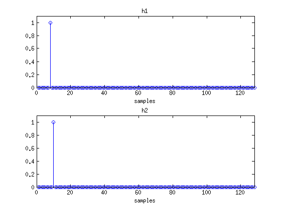
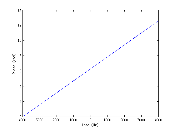
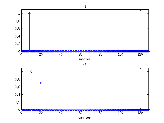
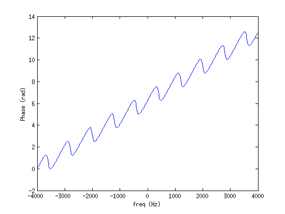
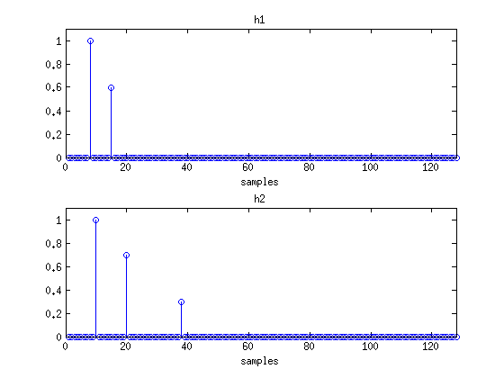
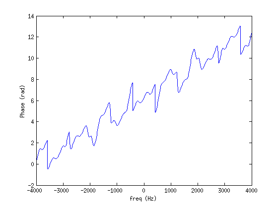
To summarize, in anechoic conditions the whitened cross-spectrum of the received wavefront consists of a linear phase component that depends on frequency f and whose slope is a function of the time difference of arrival between the wavefronts τm1,0-τm2,0. The figure below describes two impulse responses (h1 and h2) and the resulting (unwrapped) phase component of the cross-spectrum ∠Ψm(f). What is the phase component∠Ψm(f) value when the wavefront arrives at the microphones simultaneously, i.e. τm1,0=τm2,0?
Echoic model: one early arrival
Let’s now consider a case where the first microphone’s RIR is anechoic and the second microphone receives one reflected wavefront. The RIRs can be written as:
Hm1(f)=hm1,0exp(-j2πfτm1,0)
Hm2(f)=hm2,0exp(-j2πfτm2,0) + hm2,1exp(-j2πfτm2,1),
where τm2,1 is the time of flight of the reflected wavefront, and hm2,1 is the amplitude of the reflected wavefront at microphone 2. The whitened cross-spectrum of these two signals becomes
Ψm(f) = Hm1(f)H*m2(f)/(|Hm1(f)|·|Hm2(f)|)
= α0(f)·exp(-j2πf(τm1,0-τm2,0))+α1(f)·exp(-j2πf(τm1,0-τm2,1)),
where α0(f) is (hm1,0 ·hm2,0)/γ, α1(f) is (hm1,0·hm2,1)/γ, and γ=|hm1,0|·|hm2,0exp(-j2πfτm2,0) + hm2,1exp(-j2πfτm2,1)|
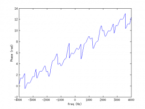
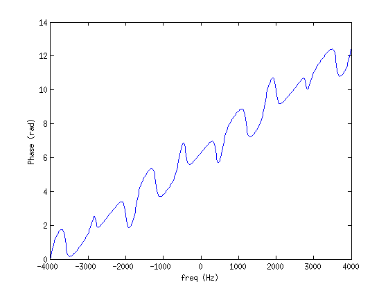
The second arrival modulates the anechoic linear phase, depending on the relative energy λ=hm2,1 / hm2,0 of the arrival, see figure above.
Echoic model: multiple arrivals
Let’s now consider two more complex cases.
- Both RIRs have one reflected path, and the whitened cross-spectrum consists of the cross-terms of each component:
Ψm(f)=α0(f)exp(-j2πf(τm1,0-τm2,0))+α1(f)exp(-j2πf(τm1,0-τm2,1))+α2(f)exp(-j2πf(τm1,1-τm2,0))+α3(f)exp(-j2πf(τm1,1-τm2,1))


- One RIR has 3 arrivals (cross-spectrum similarly consists of all cross-terms):


Question: Modify the provided Matlab script to evaluate what happens when
1) the number of taps in the RIRs is inceased;
2) the relative amplitude of the reflections is increased;
Particle filtering
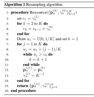
As discussed in the text, particle filtering (PF) is a tracking method suitable for using acoustic maps to estimate speaker trajectory. Several versions of PFs exist, and the basic method of “bootstrap filter” or Sequential Importance Resampling (SIR), see [1] is described in Algorithm 2 and resampling in Algorithm 1 (after [1] and [2]). An example of Matlab implementation of Algorithm 1 is available here.
Typical modeling of the target dynamics are (depending on the target state and the application scenario under investigation):
- Gaussian noise
- Langevin
[1] Arulampalam, M. S., Maskell, S., Gordon, N., & Clapp, T. (2002). A tutorial on particle filters for online nonlinear/non-Gaussian Bayesian tracking. IEEE Transactions on signal processing, 50(2), 174-188.
[2] Stone, L. D., Streit, R. L., Corwin, T. L., Bell, K. L., Bayesian Multiple Target Tracking, 2nd edition, Artec House, p.100, 2014.