
Presto-HF is a matlab toolbox, that is a collection of functions that can be called from the command line. For the moment we do not offer a graphical interface for it. Users usually develop their own one, adapted to their special needs and workflow.
We will process here the example of an 8 poles filter, implemented in wave guide dual mode technology. The coupling topology made of two quartets accommodates 4 symmetrical transmission zeros, see Dedale-libray.
We start by loading, and visualising the measurements:
>> Spbcnes0=ParseS(‘Spbcnes0.txt’);
>> PlotS(Spbcnes0);
>> PlotS(Spbcnes0,’b’);
that generate following Nyquist and Bode plots,
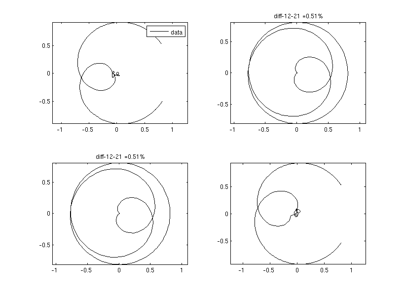
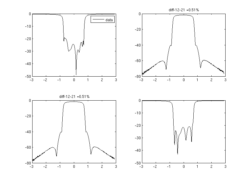
Note that the frequency has already been rescaled from the high pass Ghz domain to the low pass domain (pass-band by definition between [-1,1]).
The delay components are now extracted, and a rational model of high order is computed. This model offers a representation of the data at all frequencies: we say that it provides a completion of the original data. In red on the plot, the “completed” part.
>> Sr=CompensateDelayAndFreqShift(Spbcnes0,8);
Strategy chosen for delay. det is: causal
**********Delay [1,1]:0.007000
Start partial constraint optimisation
Start full constraint optimisation
**********Delay [2,2]:0.003000
Start partial constraint optimisation
Start full constraint optimisation
>> PlotS(Sr);

Eventually a low order rational model of order 8 is computed, shown in blue on the plot below,
>> Sr=CompFourierCoeffs(Sr);
S(1,1) ratio unstable/norme_data = 0.500036%
S(1,2) ratio unstable/norme_data = 0.010383%
S(2,1) ratio unstable/norme_data = 0.009992%
S(2,2) ratio unstable/norme_data = 0.504362%
>> Sr=RatApp(Sr,8,1);
>>PlotS(Sr);
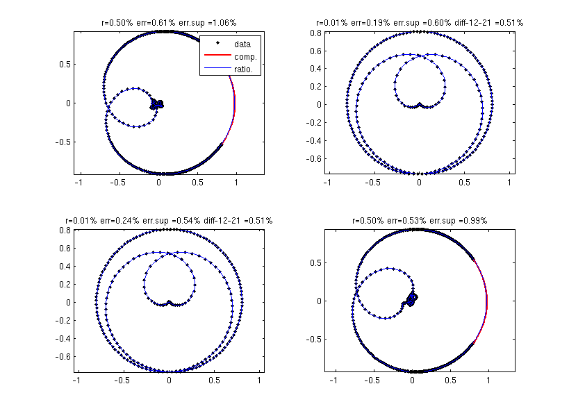 The fit between data and the rational model is excellent (the blue line corresponds to the rational approximant, the dots are the data).
The rational model is then realised as a coupled resonator circuit with a coupling topology in arrow form. The corresponding (N+2)x(N+2) coupling matrices (imaginary and real part) are shown below:
>> [M,Mred,R1,R2]=S2M(Sr);
>> disp(‘Arrow form: imag part’);imag(M)
Arrow form: imag part
ans =
0.0028 0.9126 0 -0.0000 0.0000 -0.0000 -0.0000 0.0000 -0.0000 0.0001
0.9126 -0.0418 -0.6294 -0.0000 0.0000 0.0000 -0.0000 -0.0000 -0.0003 0.0000
0.0000 -0.6294 0.0118 -0.4267 -0.0000 0.0000 0.0000 -0.0000 -0.0004 0.0000
-0.0000 -0.0000 -0.4267 0.0121 -0.3991 0.0000 -0.0000 -0.0000 -0.0333 0.0000
0.0000 0.0000 -0.0000 -0.3991 0.0189 -0.4041 0.0000 0.0000 0.0099 -0.0000
0.0000 0.0000 -0.0000 0.0000 -0.4041 0.0266 -0.2670 0.0000 0.3403 -0.0000
0.0000 0.0000 0.0000 -0.0000 -0.0000 -0.2670 -0.0765 -0.6187 -0.0626 0.0000
0.0000 0 0.0000 -0.0000 0.0000 -0.0000 -0.6187 0.1539 -0.5269 -0.0000
0.0000 -0.0003 -0.0004 -0.0333 0.0099 0.3403 -0.0626 -0.5269 0.0733 0.9222
0.0001 0.0000 0.0000 -0.0000 -0.0000 0.0000 0.0000 -0.0000 0.9222 -0.0020
>> disp(‘Arrow form: real part’);real(M)
Arrow form: real part
ans =
0.0151 0.0038 -0.0000 -0.0000 0.0000 0.0000 0.0000 0.0000 0.0001 0.0000
0.0038 0.0471 0.0033 0 0.0000 -0.0000 0.0000 -0.0000 0.0001 0.0001
0.0000 0.0033 0.0408 -0.0002 0.0000 -0.0000 -0.0000 0.0000 0.0002 -0.0000
-0.0000 0 -0.0002 0.0305 0.0004 0.0000 -0.0000 -0.0000 -0.0006 -0.0000
0.0000 -0.0000 -0.0000 0.0004 0.0232 -0.0012 -0.0000 0.0000 -0.0010 0.0000
0.0000 0.0000 -0.0000 0.0000 -0.0012 0.0247 0.0010 0.0000 -0.0002 0.0000
0.0000 0.0000 0.0000 -0.0000 -0.0000 0.0010 0.0358 -0.0020 0.0123 -0.0000
0 -0.0000 -0.0000 0 -0.0000 0.0000 -0.0020 0.0083 -0.0029 -0.0000
0.0001 0.0001 0.0002 -0.0006 -0.0010 -0.0002 0.0123 -0.0029 0.0364 -0.0005
0.0000 0.0001 -0.0000 -0.0000 0.0000 0.0000 -0.0000 -0.0000 -0.0005 0.0132
Couplings can be red directly from the imaginary part of the coupling matrix, while losses in the resonators can be red from the diagonal terms of the real part. Computation time of the whole procedure is 20 sec. on a 2.53 Ghz Intel Xeon CPU, which makes it compatible with a tuning task. When repeated tuning steps are considered on the same device, further drastic improvements of the computation time are possible, as for example the delay components needs to be identified only once.
Using Dedale the coupling can be further transformed to obtain a coupling matrix compatible with the implemented coupling topology with two quadruplets. Doing this yields two possible coupling matrices matrices, shown below in there NxN form:
M1=
-0.0418 -0.5650 0 -0.2771 0 0 0 0
-0.5650 0.0099 0.5939 0 0 0 0 0
0 0.5939 0.0212 -0.3183 0 0 0 0
-0.2771 0 -0.3183 0.0244 0.3782 0 0 0
0 0 0 0.3782 0.0217 0.3762 0 0.0810
0 0 0 0 0.3762 0.0340 0.4832 0
0 0 0 0 0 0.4832 0.0358 -0.6260
0 0 0 0 0.0810 0 -0.6260 0.0733
and
M2=
-0.0418 -0.6209 0 0.1035 0 0 0 0
-0.6209 0.0131 0.4914 0 0 0 0 0
0 0.4914 0.0205 0.3815 0 0 0 0
0.1035 0 0.3815 0.0301 0.3829 0 0 0
0 0 0 0.3829 0.0219 -0.3233 0 -0.2450
0 0 0 0 -0.3233 0.0236 0.5779 0
0 0 0 0 0 0.5779 0.0376 -0.5818
0 0 0 0 -0.2450 0 -0.5818 0.0733
This ambiguity is intrinsic to the use of this coupling topology, and corresponds to the different ways to affect the two symmetric pairs of zero to the two quadruplets. Knowing for example that on the hardware under tuning, the most outer (in frequency w.r to the passband) pair of zeros is controlled by the first quadruplet, allows to conclude that M2 is the coupling matrix implemented by the filter.