1. Description
This case study is closely based on the one presented in [KNP04,KNP07] but contains much more components. The system consists of an input processor (I) connected to 50 groups of 3 sensors, an output processor (O), connected to 30 groups of 2 actuators, and a main processor (M), that communicates with I and O through a bus. At every cycle, 1 minute, the main processor polls data from the input processor that reads and processes data from the sensor groups. Based on this data, the main processor constructs commands to be passed to the output processor for controlling the actuator groups.
The reliability of the system is affected by the failures of the sensors, actuators, and processors. The probability of bus failure is negligible, hence we do not consider it. The sensors and actuators are used in 37-of-50 and 27-of-30 modular redundancies, respectively. That means if at least 37 sensor groups are functional (a sensor group is functional if at least 2 of the 3 sensors are functional), the system has enough information to function properly. Otherwise, the main processor is reported to shut the system down. In the same way, the system requires at least 27 functional actuator groups to function properly (a actuator group is functional if at least 1 of the 2 actuators is functional). Transient and permanent faults can occur in processors I or O and prevent the main processor M to read data from I or send commands to O. In that case, M skips the current cycle. If the number of continuously skipped cycles exceeds the limit K, the processor M shuts the system down. When a transient fault occurs in a processor, rebooting the processor repairs the fault. Lastly, if the main processor fails, the system is automatically shut down. The mean times to failure for the sensors, the actuators, and the processors are 1 month, 2 months and 1 year, respectively. The mean time to transient failure is 1 day and I/O processors take 30 seconds, 1 time unit, to reboot.
2. Implementation
The reliability of each component in the system is modeled as a Continuous-Time Markov Chain (CTMC) that is realized in SystemC, in which a sensor group has 4 states (0, 1, 2, 3, the number of working sensors), 3 states (0, 1, 2, the number of working actuators) for an actuator group, 2 states for the main processor (0: failure, 1: functional), and 3 states for I/O processors (0: failure, 1: transient failure, 2: functional). A state of the CTMC is represented as a tuple of the component’s states, and the mean times to failure define the delay before which a transition between states is enabled. The delay is sampled from a negative exponential distribution with parameter equal to the corresponding mean time to failure. Hence, the model has about 2^155 states comparing to the model in [KNP07] with about 2^10 states, that makes the PMC technique is unfeasible. That means the state explosion likely occurs, even with some abstraction, i.e., symbolic model checking is applied.
Source code and automated shell scripts – control_system.tar.gz
3. Experimental results
We define four types of failures: failure_1 is the failure of the sensors, failure_2 is the failure of the actuators, failure_3 is the failure of the I/O processors and failure_4 is the failure of the main processor. For example, failure_1 is defined by (number_sensors < 37) and (proci_status = 2). It specifies that the number of working sensor groups has decreased below 37 and the input processor is functional, so that it can report the failure to the main processor. We define failure_2, failure_3, and failure_4 in a similar way. In our analysis which is based on the one in [KNP07] with K = 4, in which the properties are checked every 1 time unit.
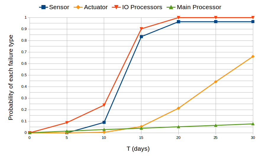
First, we study the probability that each of the four types of failure eventually occurs in the first T time of operation. This is done using the BLTL formula F <= T (failure_i). The following figure plots these probabilities over the first 30 days of operation. We observe that the probabilities that the sensors and I/O processors eventually fail are more than the others do. In the long run, they are almost the same and approximate to 1, meaning that the sensors and I/O processors will eventually fail with probability 1. The main processor has the smallest probability to eventually fail.
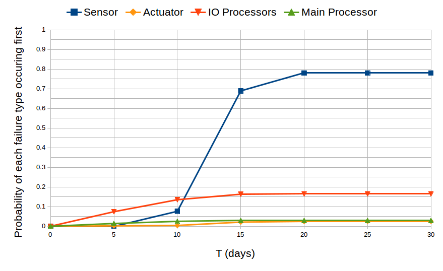
Second, we try to determine which kind of component is more likely to cause the failure of the system, meaning that we determine the probability that a failure related to a given component occurs before any other failures. The atomic proposition (shutdown = \/ failure_i) indicates that the system has shut down because one of the failures has occurred, and the BLTL formula (not shutdown U<= T failure_i) states that the failure i occurs within T time units and no other failures have occurred before the failure i occurs. The figure shows the probability that each kind of failure occurs first over a period of 30 days of operation. It is obvious that the sensors are likelier to cause a system shutdown. At T=20 days, it seems that we reached a stationary distribution indicating for each kind of component the probability that it is responsible for the failure of the system.
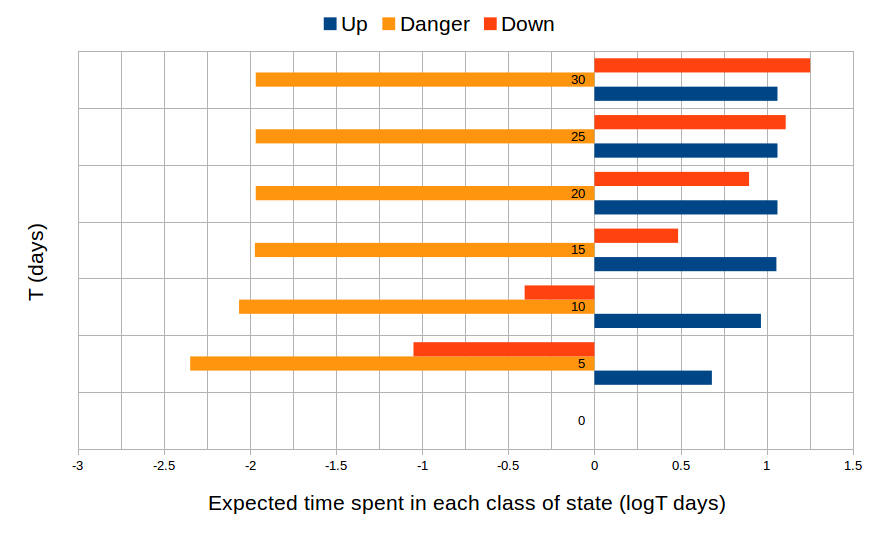
For the third part of our analysis, we divide the states of system into three classes: “up”, where every component is functional, “danger”, where a failure has occurred but the system has not yet shut down (e.g., the I/O processors have just had a transient failure but they have rebooted in time), and “shutdown”, where the system has shut down. We aim to compute the expected time spent in each class of states by the system over a period of T time units. To this end, we add in the model, for each class of state c, a random variable reward_c that measures the time spent in the class c.
In our tool, the formula X<=T reward_c returns the mean value of reward_c after T time of execution. The results are plotted in the following figure. From T=20 days, it seems that the amounts of time spent in the “up” and “danger” states are converged at 10^1.063 = 11.57 days and 10^-1.967 = 0.01 days, respectively.
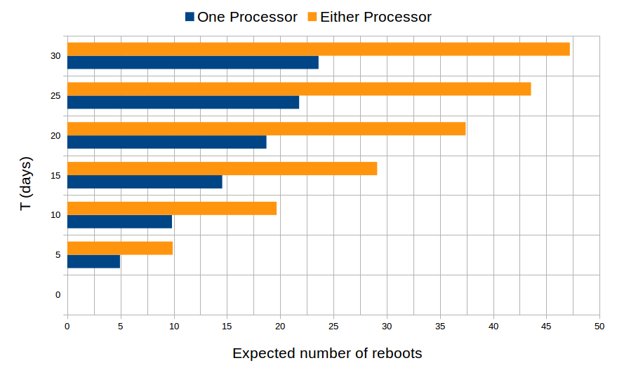
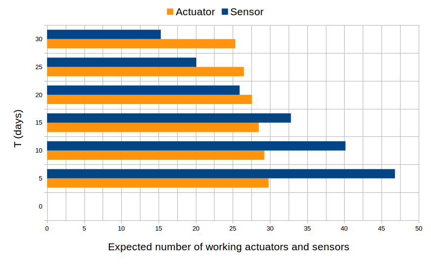
Finally, we approximate the number of reboots of the I/O processors, and the number sensor groups, actuator groups that are functional over time by computing the expected values of random variables that count the number of reboots, functional sensor and actuator groups. The results are plotted in the following figures. It is obvious that the number of reboots of both processors doubles the number of reboots of each processor since they have the same behavior.