Description
We use SystemC with GNU Scientific Library (GSL) to model a large embedded control system in terms of the number of components (i.e., in case the CTMCs with 4 and 3 states are used to model the groups of 3 sensors and 2 actuators, respectively, our model has about 2^155 states. The system consists of an input processor (I), connected to 50 groups of 3 sensors (from S1 to S50), an output processor (O), connected to 30 groups of 2 actuators (from A1 to A30), and a main processor (M), communicates with I and O through a bus that is shown in Fig. 1.
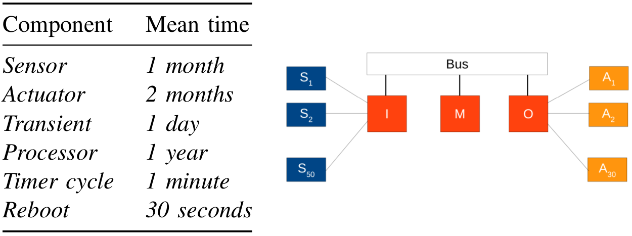
Fig. 1: An Embedded Control System and the Mean Times to Failure
Every cycle controlled by a timer in the main processor (i.e., 2 units of time), the main processor polls the input processor that reads and processes data from the sensors. It is then elaborates the results from the input processor into commands to be passed to the output processor, which controls the actuators. For instance, the data can be fluid level, temperature, or pressure of the environment, while the commands sent to actuators could be used for controlling valves. The reliability of the system is affected by the failures of the sensors, actuators, and processors (the probability of bus failure is negligible, hence it is not considered explicitly). The sensors and actuators are used in 37-of-50 and 27-of-30 modular redundancy, respectively. Hence if the number working sensor groups is equal or more than 37 (a sensor group is functional if at least two of the three sensors are functional), the input processor can determine sufficient information to process. Otherwise, the main processor is reported to shut the system down. In the same way, the system can be functional with the failure of less than 3 actuator groups (a actuator group is functional if at least one of the two actuators is functional). The I/O processors can have a transient fault or a permanent fault and make the main processor unable to read data from I or send commands to O, then M skips the current cycle. If the number of continuously skipped cycles exceeds a limit, K, M then shuts the system down. When a processor has a transient fault, it can be refined automatically by the processor reboot. Lastly, if the main processor fail, the system is automatically shut down. The mean times to failure for the sensors, actuators, I/O processors, main processor, and the mean times for the delays are given in Fig. 1 with the time unit is 30 seconds.
SystemC Model
All components can be modelled as CTMCs and their mean times to delays are distributed exponentially. Each component of the system is implemented by a module in SystemC, 50 for the sensor groups, 30 for the actuator groups, one for each processor, and one for the bus. For instance, the following implementation of a CTMC which models a group of 3 sensors, where s = 0,…3 is the number of working sensors in the group and the holding time in the current state ht is a continuous strictly positive random variable, which has an exponential distribution at rate s*lambda. At any time if there exists some working sensor (s > 0), a single sensor can fail and the number of working sensor is decreased by 1 by the statement (s = s – 1).
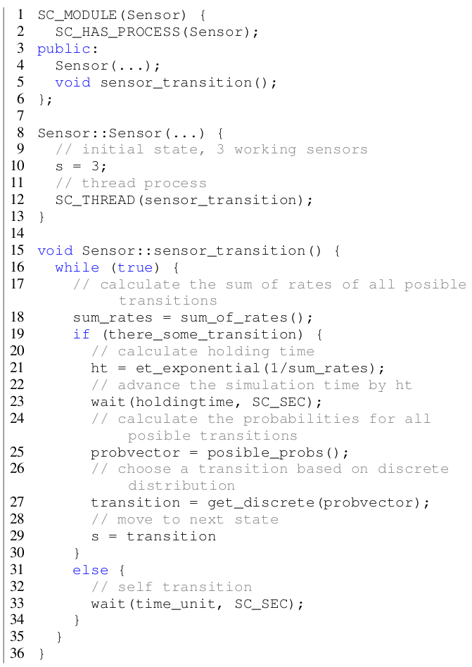
Fig. 2: Sensor Group Implementation in SystemC
The modules modelling the actuators, the I/O processor, and the main processor are done in the same way as the module for the sensors. However, one point of note is the implementation of the communication between the processors via the connecting bus. The connecting bus comprises 3 input ports which are connected to the output ports of the input processor, output processor, and the main processor by 3 SystemC buffer signals to synchronize actions between the processors. For example, when the input processor has a transient fault, as soon as it reboots successfully, it sends the notification to the main processor through its output port. In the similar fashion, the output processor notifies the main processor of its reboot and the main processor notifies its time-out when the number of continuously skipped cycles exceeds the limit K, as soon as they occur. All the synchronized actions when receiving these notifications are implemented in the connecting bus module.
- SystemC Model – ecs_src.tar.gz
- Instrumented Model – ecs_instrumented.tar.gz
- Plasma Project – ecs_plasma.tar.gz
Analysis Results
The above verification framework has used to analyze a set of dependability properties. The set of observed variables, the temporal resolution and their meaning are given in following table. There are four types of failure, denoted by failure_i, where i = 1…4, which can make the system shut-down: failure of the sensors, the actuators, the I/O processors, and the main processor. In our analysis with K = 4, we applied the Monte Carlo simulation with 3000 samples. First, we study the probability that each of the four types of failure eventually occurs in the first T time of operation. This is done using the BLTL formula F <= T (failure_i).
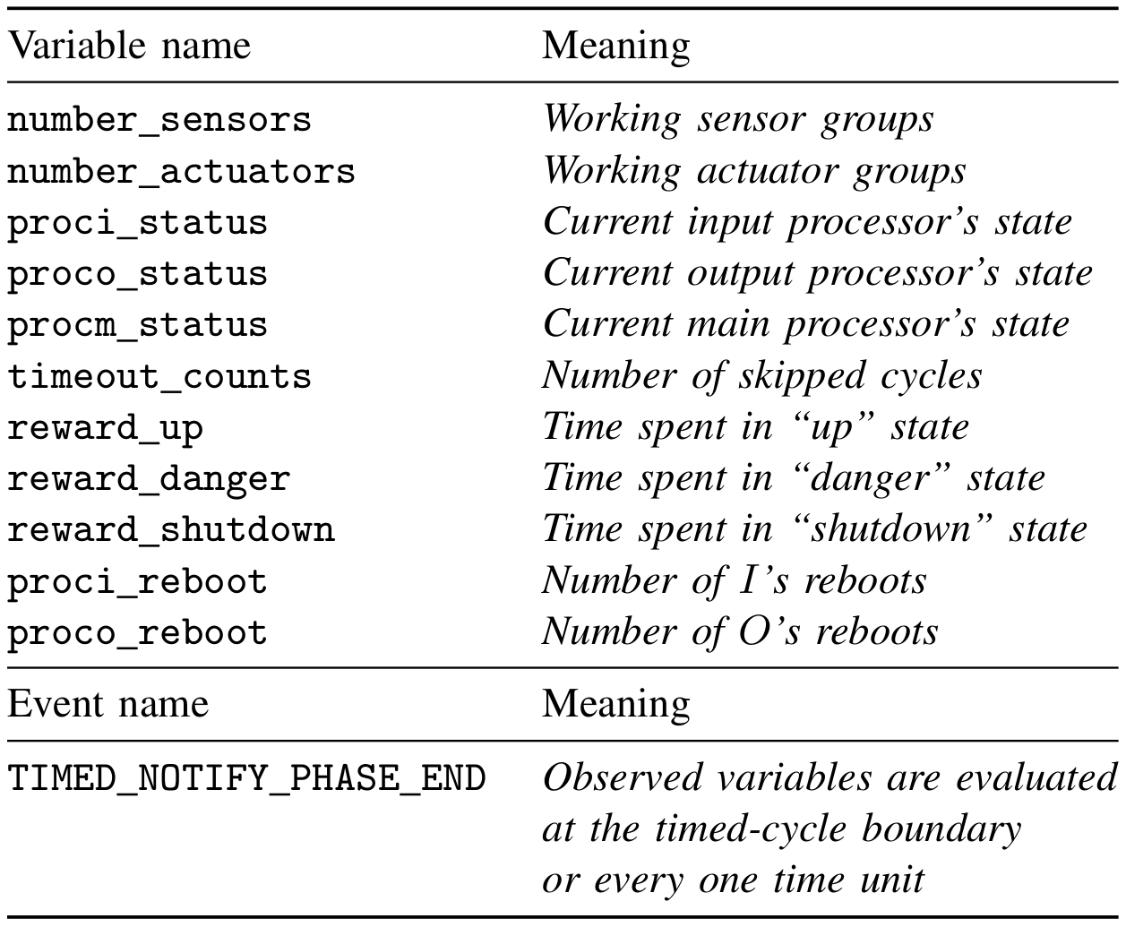
Table 1: Observed Variables and Time Resolution
The atomic propositions such as failure_i are predicates over the observed variables from the generated monitor. For example, the failure of more than 10 sensor groups, failure_1, is defined by the following predicate (number_sensors < 37 and proci_status = 2). It specifies that the number of working sensor groups has decreased below 37 and the input processor is functioning, thus it can report the failure to the main processor. We do the same for failure_2, failure_3, and failure_4 over the observed variables. Figure 3 plots these probabilities over the first 30 days of operation. We observe that the probabilities that the sensors and I/O processors eventually fail are more than the others do. In the long run, they are almost the same and approximate to 1, meaning that the sensors and I/O processors will eventually fail with probability 1. The main processor has the smallest probability to eventually fail.
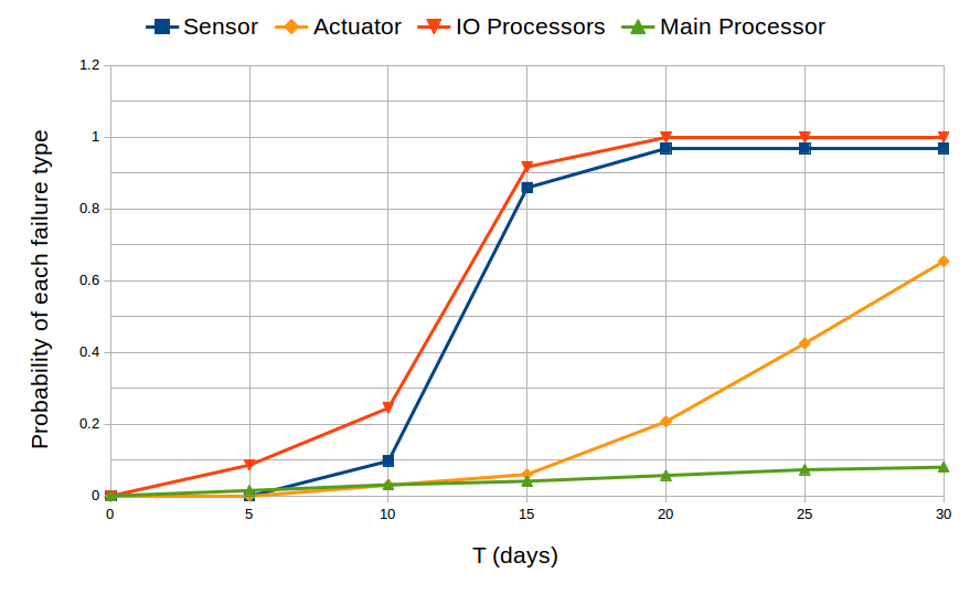
Fig. 3: The probability that each of the 4 failure types in the first T time of operation
For the second part of our analysis, we show how non-trivial properties can be can be expressed using “until” temporal operator. Consider a situation that a sensor fails, the actuators are unaware of this failure. They will continue to operate and might eventually fail. Hence, it is necessary to determine the probability that one failure occurs before any other failures. The formula (not shutdown U <= T failure_i) denotes that the failure i occurs within T time units and no other failure has occurred before the failure i occurs. The atomic proposition shutdown which indicates that the system has shut-down, meaning that one of the failures has occurred, is defined by (failure_1 or failure_2 or failure_3 or failure_4). Figure 4 shows these probabilities over a period of 30 days of operation. It is obvious that the sensors are more likely to cause a system shutdown. In the long run (e.g., as T to infinity), the sum of these probabilities is exactly 1, i.e., the system will eventually shut down with probability 1. In our experiment, this sum is statistically computed and approximates to 1. It can be seen, for example, when the period of operation longer than 20 days the probability that system will eventually shut down is almost 1 (e.g., 0.793 + 0.150 + 0.030 + 0.025 = 0.998 at T = 20 days).
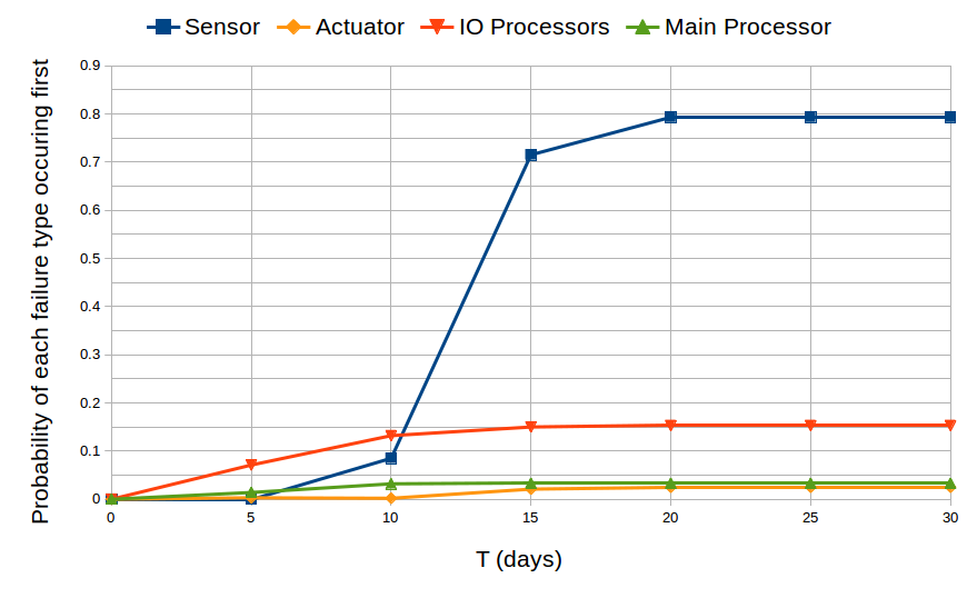
Fig. 4: The probability that each of the 4 failure types is the cause of system shutdown in the first T time of operation
For the third part of our analysis, we divide the states of system into three classes: “up”, where every component is functioning, “danger”, where a failure has occurred but the system has not yet shut down (e.g., the I/O processor have just had a transient failure but they have rebooted in time then the M processor has yet to detect this), and “shutdown”, where the system has shut down. Our intention is computing the expected time spent in each class of states by the system over a period of T time units. The results are plotted in Figure 5.
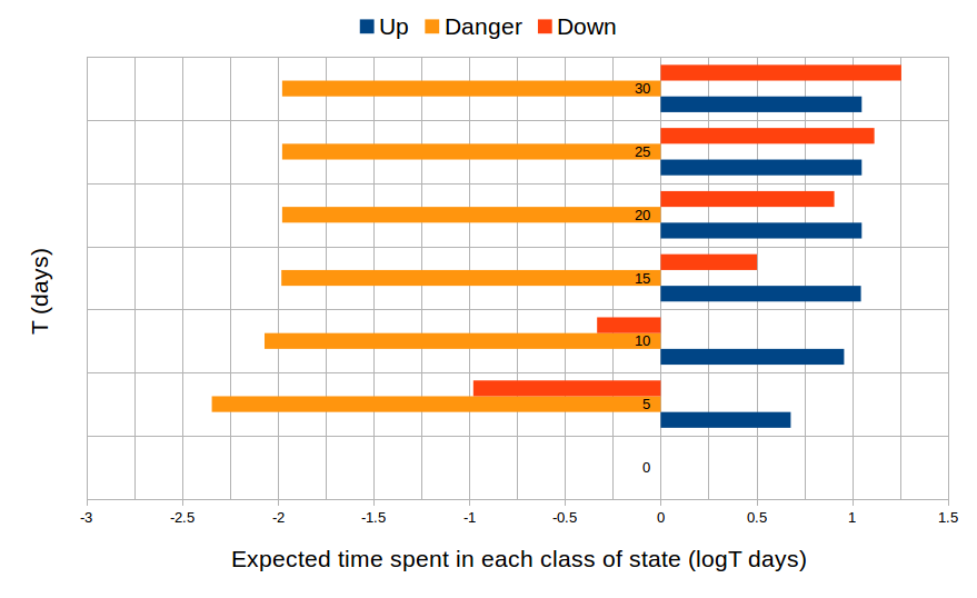
Fig. 5: The expected amount of time spent in each of the states: “up”, “danger” and “shutdown”
Finally, we approximate the number of input, output processor reboots which occur and the number sensor groups, actuator groups that are functional over time by computing the expected values of random variables that count the number of reboots, functional sensor and actuator groups. The results are plotted in Figure 6 and Figure 7.
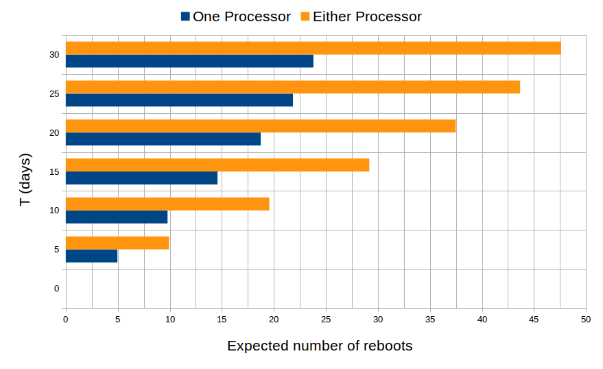
Fig. 6: Expected number of reboots that occur in the first T time of operation
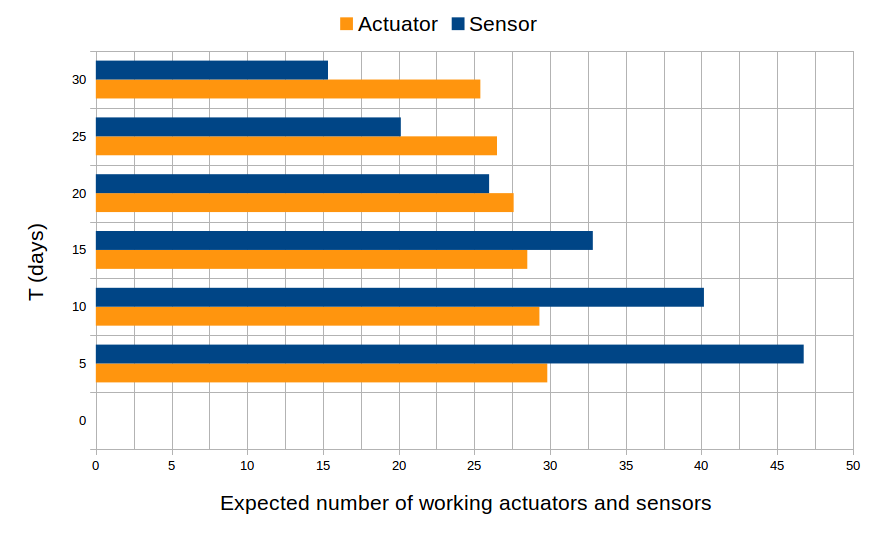
Fig. 7: Expected number of reboots that occur in the first T time of operation