
Contents
The broadband matching problem aims to minimise within a specified frequency interval I the reflected power from the system (\(S\)) composed of a matching filter (\(F\)) cascaded with load (\(A\)). Note that the load is represented here as a two port device.
Statement of the general matching problem
The problem is stated in its general form as the minimisation over the filter \(F\) of the maximum in the band of \(|S_{11}(\omega)|\) over the frequency variable \(\omega\). If the filter is parametrised in function of its reflection parameter \(F_{22}\), the only constraint imposed is that the reflection \(F_{22}\) must remain passive and stable. Therefore \(F_{22}\) is a stable function with \(|F_{22}|\leq 1\) on the whole frequency axis.
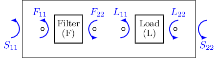
Schematic of the global system with input and output reflection of each device
Chaining operation
The scattering parameter \(S_{11}\) can be computed by the chain operation (\(F\circ A_{11}\)):
\(\displaystyle S_{11} =F\circ A_{11}= F_{11} + \frac{F_{21}F_{12}A_{11}}{1-F_{22}A_{11}} \)
where \(F_{12},F_{21}\) stand for the transmission parameters of the matching filter.
For a lossless device, the scattering matrix is unitary, this means \(S\cdot S^* = I\) (\(S^*(\omega) \equiv \overline{S(\overline{\omega})}\)). Using this property we can express:
\(\displaystyle|S_{11}| = \left|\frac{F_{22}^*-A_{11}}{1-F_{22}A_{11}} \right|\)
This expression correspond to the pseudohyperbolic distance between the function \(F_{22}^*\) and \(A_{11}\).
Optimisation over the Schur functions
The problem is stated then as the minimisation of the previous pseudohyperbolic distance over the functions \(F_{22}\) that are passive and stable.
The functions \(F_{22}\) that are passive (\(|F_{22}(\omega)|<=1\)) and stable (analytic) in a domain are called schur functions. We denote the set of such functions by \(\mathbb{B}\).
Thus the aim is to solve:
\(\displaystyle\underset{F_{22}\in \mathbb{B}}{\text{min}}\underset{\omega}{\text{max}}\left|\frac{F_{22}^*(\omega)-A_{11}(\omega)}{1-F_{22}(\omega)A_{11}(\omega)} \right|\)
for all \( \omega\) in the passband.
Infinite dimension solution
If the only restriction of the function \(F_{22}\) is being stable and passible (without limitation on the degree), the previous problem can be solved optimally. This is possible because the set \( \mathbb{B}\) is a convex set.
The optimal solution to the general problem was already obtained by Helton in [ref]. He computed, for a given load \( A_{11}\) the function \( S_{22}\) that provides a reflection \( S_{11}\) lowest possible absolute value within the passband. This reflection level, being obtained without limitation on the degree of \(F_{22}\), represents a lower bound on the reflection level that can be obtained for \( A_{11}\). We can see an example of the Helton bound for a particular load in the following picture, along with the function \( F_{22}\) of infinite degree providing the optimal reflection level.
However, if the function \( F_{22}\) is constrained to be rational with a low degree, this bound will not be accurate. Symilarly, the optimal rational function \( F_{22}\) with a given low degree will differ from the one obtained with no degree limitation.
Rational matching problem
If we now restrict the function \( F_{22}\) only to be rational, i.e. \( F_{22}(\omega)=\frac{p(\omega)}{q(\omega)}\) with \(p\) and \(q\) polynomials of degree at most N, the previous problem becomes too difficult to solve. Intead we use a parametrisation allowing for the transmission zeros to be prescribed as well.
Belevitch representation
We use the belevitch form to parametrise the global system:
\(\displaystyle S = \frac{1}{q}\left(\begin{array}{cc}\epsilon p^* & -\epsilon r^* \\ r & p \end{array} \right)\)
with \(\epsilon\)a uni-modular constant, and \(q,p,r\) polynomials of degree at most N satisfying \(qq^*=pp^*+rr^*\) with \(p^*(\omega)=\overline{p(\overline{\omega})}\). Note that q is a stable polynomial (analytic in the stability domain). Additionally, the polynomial \(r\) is fix by the user.
This parametrisation is customary in classical filter design where the belevitch form is used to parametrise lossless devices. Similarly the transmission zeros are often set to given positions in the complex plane, usually with the purpose of increasing the out-of-band selectivity or to have some control on the group delay in the passband.
Feasible responses
Now given the chaining operation introduced before:
\(\displaystyle S_{22} =F_{22}\circ A = A_{22} + \frac{A_{21}F_{22}A_{21}}{1-A_{11}F_{22}}\)
we define the set of feasible functions (\(\mathbb{F}\)) as the image of the schur functions (\(\mathbb{B}\)) under the chaining application:
\(\displaystyle \begin{array}{lll}\mathbb{B} & \longrightarrow &\mathbb{F} \\ F_{22} & \longrightarrow& S_{22}=F_{22}\circ A \end{array}\)
In other words, a function \(S_{22}\) is feasible for a given load \(A\) if and only if there exists a Schur function \(F_{22}\) such that \(F_{22}\circ A = S_{22}\).
Rational matching with prescribed transmission zeros
With S being parametrised in the belevitch form as before, we denote by \(\mathbb{F}^N_R\) the set admissible functions \(S_{22}=\frac{p}{q}\) satisfying \(qq^* – pp^* = R \) (the set of rational responses where the transmission zeros are prescribed).
With those definitions, the rational matching problem can be stated as the minimisation in the passband of the reflection of the global system knowing that there must exist a function \(F_{22}\) rational of given degree that chained to the load provides the desired reflection:
\(\displaystyle\underset{S_{22}\in \mathbb{F}^N_R}{\text{min}}\underset{\omega}{\text{max}}\left|S_{22}(\omega) \right|\)
for all \( \omega\) in the passband.
Note that the problem is stated here on \(|S_{22}|\) instead of \(|S_{11}|\). However, it is not relevant since for lossless systems and \(\omega\) real, \(|S_{11}(\omega)| = |S_{22}(\omega)|\).
The Fano/Youla characterisation
Having defined the set of feasible responses \(S_{22}\in \mathbb{F}\) as the reflection parameters that can be obtained by connecting a passive stable device to a prescribe load, we need a charactesation for it. In other words, what requisites must be satisfied by a reflection \(S_{22}\) to be feasible?, of course we know that the requisite is that there must exist a passive stable filter F such that the cascade of that filter with the load shows the reflection \(S_{22}\) at the second port. However thats too abstract.
A better characterisation can be obtained from the chaining equation
\(\displaystyle S_{22} = A_{22} + \frac{A_{21}A_{12}F_{22}}{1-F_{22}A_{11}} \)
We look at the transmission zeros of the load \(\alpha_i\) (the points inside the stability domain of the complex plane for which \(A_{21}(\alpha_i)A_{12}(\alpha_i) = 0\). At those points, for any passibe stable filter F the right term in the previous equation vanishes since the denominator can not be zero inside the stability domain. Therefore we obtain the interpolation condition
\(S_{22}(\alpha_i) = A_{22}(\alpha_i)\)
This is a necessary condition for a function \(S_{22}\) to be feasible. In addition, as the main result of Fano/Youla work, it was shown that this condition is indeed necessary and sufficient.
(this stand for the case of simple transmission zeros of the load inside the complex plane, if the load has either transmission zeros of higher multiplicity or transmission zeros on the frequency axis, the previous condition has to be modified including equalities on the derivatives as well).
In conclussion, if a response \(S_{22}\) satisfied the previous conditions for a given load A then it exist a passive stable filter F that chained with the load provides the reflection \(S_{22}\) at the second port (the function \(S_{22}\) is feasible).
Thus this interpolation conditions represent a characterisation of the feasible responses \(\mathbb{F}\).
Nevanlinna-Pick interpolation
The last tool required to understand how puma works is the Nevanlinna-Pick interplation theorem, it states:
Given N points \(\alpha_1,\alpha_2,\cdots, \alpha_N\) in the lower half of the complex plane (points with negative imaginary part), and N complex values \(\gamma_1,\gamma_2,\cdots, \gamma_N\) with \(|\gamma_i|<1\), there exist a schur function \(S_{22}\) (passive stable in the lower half plane) such that \( S_{22}(\alpha_i)=\gamma_i\) if and only if the followig matrix is positive definite.
\(\displaystyle \frac{1}{j}\left(\begin{array}{cccc}\frac{1-|\gamma_1|^2}{2j\text{Im}(\alpha_1)} & \frac{1-\gamma_1\overline{\gamma_2}}{\alpha_1 – \overline{\alpha_2}} & \cdots & \frac{1-\gamma_1\overline{\gamma_N}}{\alpha_1 – \overline{\alpha_N}}\\ \frac{1-\gamma_2\overline{\gamma_1}}{\alpha_2 – \overline{\alpha_1}} & \frac{1-|\gamma_2|^2}{2j\text{Im}(\alpha_2)} & \cdots & \frac{1-\gamma_2\overline{\gamma_N}}{\alpha_2 – \overline{\alpha_N}} \\ \vdots & \vdots & \ddots & \vdots\\ \frac{1-\gamma_N \overline{\gamma_1}}{\alpha_N -\overline{\alpha_1}} & \frac{1-\gamma_N\overline{\gamma_2}}{\alpha_N-\overline{\alpha_2}}& \cdots & \frac{1-|\gamma_N|^2}{2j\text{Im}(\alpha_N)}\end{array} \right)\)
This matrix is called the Pick matrix.
Nevanlinna parametrisation
Nevanlinna also provided a parametrisation of all solutions to the interpolation problem \( S_{22}(\alpha_i)=\gamma_i\) with \(S_{22}\in \mathbb{B}\) (schur functions). In the general case, when the pick matrix is positive definite (with N interpolation conditions)
\(\displaystyle S_{22}(\omega) = \frac{\Theta_1(\omega) + \Theta_2(\omega)f(\omega)}{\Theta_3(\omega) + \Theta_4(\omega)f(\omega)}\)
where \(\Theta_i(\omega)\) are polynomials of degree at most N and \(f(\omega)\) is a schur function.
Remark: in our context, this expression is actually equivalent to the chaininig operation \(f\circ A\) where the \(\Theta_i\) polynomials are in fact the polynomials involved in the belevitch model of the load \(A\).
In the particular case where the pick matrix is positive semi-definite and singular, there is a unique solution to the interpolation problem in the form of a blaschke product \(b(\omega)\in\mathbb{B}\):
\(\displaystyle b(\omega) = e^{j\phi}\prod_{i=1}^M \frac{\omega – \beta_i}{\omega-\overline{\beta_i}}\)
where M stand for the rank of the pick matrix, \(\beta_i\) belong to the analicity domain and with \(\phi\) real.