Algorithms

Rational H2 approximation

Given a matrix-valued function $F(z)$ whose entries are assumed to be in the Hardy space ¹ $H^2$ and a positive integer n, the problem is to find a stable² rational matrix $H(z)$ of McMillan degree³ at most n which minimizes the $L^2$ norm

$\|F-H\|_2^2=\frac{1}{2\pi} {\rm Tr} \int_0^{2\pi}(F-H)(e^{it}) {(F-H)(e^{it})}^*dt.$ It is known [1] that a global minimum does exist and has exact degree n unless $F(z)$ is of lower degree. Moreover, if $F(z)$ has degree n, then the only critical point of the criterion is $F(z)$ itself [2]. The approach used in RARL2 was first developped for scalar functions [3] and then in the matrix case [4].

1. Hardy spaces: the space $L^2$ of square integrable functions on the unit disk splits into two orthogonal subspaces: the space $H^2$ of $L^2$ functions having an analytic continuation in the unit disk (negative Fourier coefficients are zero) and the space $H_-^2$ of $L^2$ functions having an analytic continuation outside the unit disk and vanishing at infinity (non-negative Fourier coefficients are zero)

2. stable: poles inside the unit disk

3. McMillan degree: size of the A-matrix in a minimal realization/ number of poles counting multiplicity

Reduction of the optimization space

We use a special matrix fraction description known has Douglas-Shapiro-Shields factorization, and write a rational matrix of degree n as

$H= G C$ where $G(z)$ is a lossless matrix⁴, of same McMillan degree than $H(z)$ , and $C(z)$ is an anti-stable matrix.

$H(z)$ and $G(z)$ : same observable pair $(C,A)$
$G(z)$ and $(C,A)$ bring the (left) pole structure
unique up to a unitary matrix
right generalization of an irreducible rational fraction

By the Hilbert projection theorem , at a local minimum $H(z)$ of the criterion, $C(z)$ has to be the projection $P^+$ of $G^{-1}F$ onto $H^2$ . The approximation problem reduces to the minimization of a concentrated criterion [4,5]

$G \mapsto \|F-G\,P^+(G^{-1}F)\|^2$
over the (quotient) set of lossless matrices of McMillan degree n up to a right unitary matrix.

Advantage: minimization over a bounded set

4. lossless matrix: rationnal matrix analytic outside the unit disk which takes unitary values on the circle.

State-space formulas

In practice, the concentrated criterion is computed using balanced realizations⁵ to represent lossless matrix functions. We have the nice following property

$\left\{\begin{array}{cl} D+C(zI-A)^{-1}B &\hbox{ lossless }\\ (A,B,C,D) &\hbox{ balanced }\end{array}\right. \Leftrightarrow \begin{bmatrix} D & C \\ B & A \end{bmatrix} \hbox{ unitary }$

Write the state-space realization of $F(z)$ and $H(z)$ .
$F(z)= {\cal C} (zI- {\cal A})^{-1} {\cal B}~~~ H(z)={C}(zI-{ A})^{-1}{\hat B}$
where the pair $(C,A)$ is assumed output normal : $A^*A+C^*C=I$
The Hilbert projection property translates into the classical necessary conditions for optimality
${\hat B}=-{\cal Q}^*{\cal B}~~~ \hbox{ where }~~~ {\cal A}^* {\cal Q} A +{\cal C}^* C= {\cal Q}.$
The concentrated criterion becomes
$J(A,C)=\|F\|_2^2-\hbox{Tr}({\cal B}^* {\cal Q}{\cal Q}^* {\cal B})$
defined over the set of equivalence classes under similarity of balanced output pairs (BOP) .

Advantage: computation with unitary matrices

5. A balanced realization is such that both grammians are equal and diagonal

Parametrization of the optimization space

The optimization space has a manifold structure [6]. We use an atlas of charts, like for the earth, where each chart provides a local flat (Euclidien) representation which allows for the use of differential tools. In the actual version of RARL2, we use the atlas presented in [7], called lossless mutual encoding

A chart is indexed by a lossless matrix/unitary realization $(W,X,Y,Z)$
A BOP, given by a unitary realization $(A,B,C,D)$ can be parametrized in this chart iff the solution $\Sigma$ to
$\Sigma - A^* \Sigma W = C^* Y$
is positive definite.
The BOP is represented in the chart by the parameters matrix
$V= D^*Y+B^*\Sigma W$

Advantage: use of differential tools safe

Optimization over a manifold

In RARL2, the minimization process makes use of the Matlab solver fmincon.
The optimization is carried over the manifold structure as illustrated below:

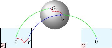
Initialization: $G_0(z)\equiv (A_0,B_0,C_0,D_0)$ computed by balanced truncation [Kun, Lin, 1981]
Optimization with respect to the local coordinates $V$ using fmincon
Change of chart handled by a non-linear constraint:
$\mbox{min eig} ~\Sigma \leq \epsilon \rightsquigarrow \mbox{change chart}$
Changing chart is easy: adapted chart at $G(z):~ V=0$

References

[1] L. Baratchart, Existence and generic properties for L2 approximants of linear systems I.M.A. Journal of Math. Control and Identification 3, 89-101 (1986)

[2]L. Baratchart and M. Olivi Critical points and error rank in matrix H2 rational approximation and the strong differential consistency of output error identification from white noise inputsConstructive Approximation 14, pp. 273-300 (1998)

[3] L. Baratchart, M. Cardelli, M. Olivi, Identification and rational L2 approximation: a gradient algorithm, Automatica 27(2) 413-418 (1991)

[4] P. Fulcheri and M. Olivi Matrix rational H2 approximation: a gradient algorithm based on Schur analysis SIAM Journal on Control and Optimization Vol. 36, No. 6, 2103-2127(1998)

[5] M. Olivi, F. Seyfert, J.P. Marmorat, Identication of microwave filters by analytic and rational H²approximation, Automatica, 49, 317-325(2013)

[6] D. Alpay, L. Baratchart, A. Gombani, On the differential structure of matrix-valued rational inner functions, Operator Theory: Advances and Applications, 73, 30–66(1994)

[7] J.P. Marmorat, M. Olivi, Nudelman Interpolation, Parametrization of Lossless Functions and balanced realizations, Automatica, 43 , 1329-1338(2007)

Rational H2 approximation

Reduction of the optimization space

State-space formulas

Parametrization of the optimization space

Optimization over a manifold

References