
WiFi is probably the most popular short-range wireless access technology with an exponential increase of Access Points (AP) deployments for the past few years [1]. They are being deployed in companies, schools, public and private areas; resulting in a high APs density and overlapping coverage areas. Usually all APs are switched on all the time, even when the number of users served by the wireless access network is very low, resulting in a high and partially wasteful energy consumption. Even though a single AP consumes only few watts, the total energy consumed could reach hundreds of watts in large deployments. For example, according to [2] the ADSL boxes (which are usually APs too) in France consume 5TWh per year. Tsui et al. [3] detected over 103000 APs in the city of Taipei through war-walking, while Achtzehn et al. [4] estimated the density of APs deployed in different cities in Germany to vary between 488 AP per km2 in industrial areas, and 6103 AP per km2 in urban residential areas. Faced by AP proliferation and with the goal of reducing the energy consumption, recent research efforts have proposed algorithms to dynamically switch on and off a set of APs depending on the traffic load.
In continuity with these efforts, we study the Wifi AP deployment in an urban environment and evaluate the AP redundancy in providing network coverage. We provide a methodology and a set of tools to measure this density. Using the Android application Wi2Me to performs network scanning, we gather real data about APs through war-walking in the centre of Rennes – France. After processing these data with various filters, we apply two different selection algorithms to select a minimal set of APs that are enough to provide the same coverage, assuming that the non-selected APs could be switched off.
Description of the experiment
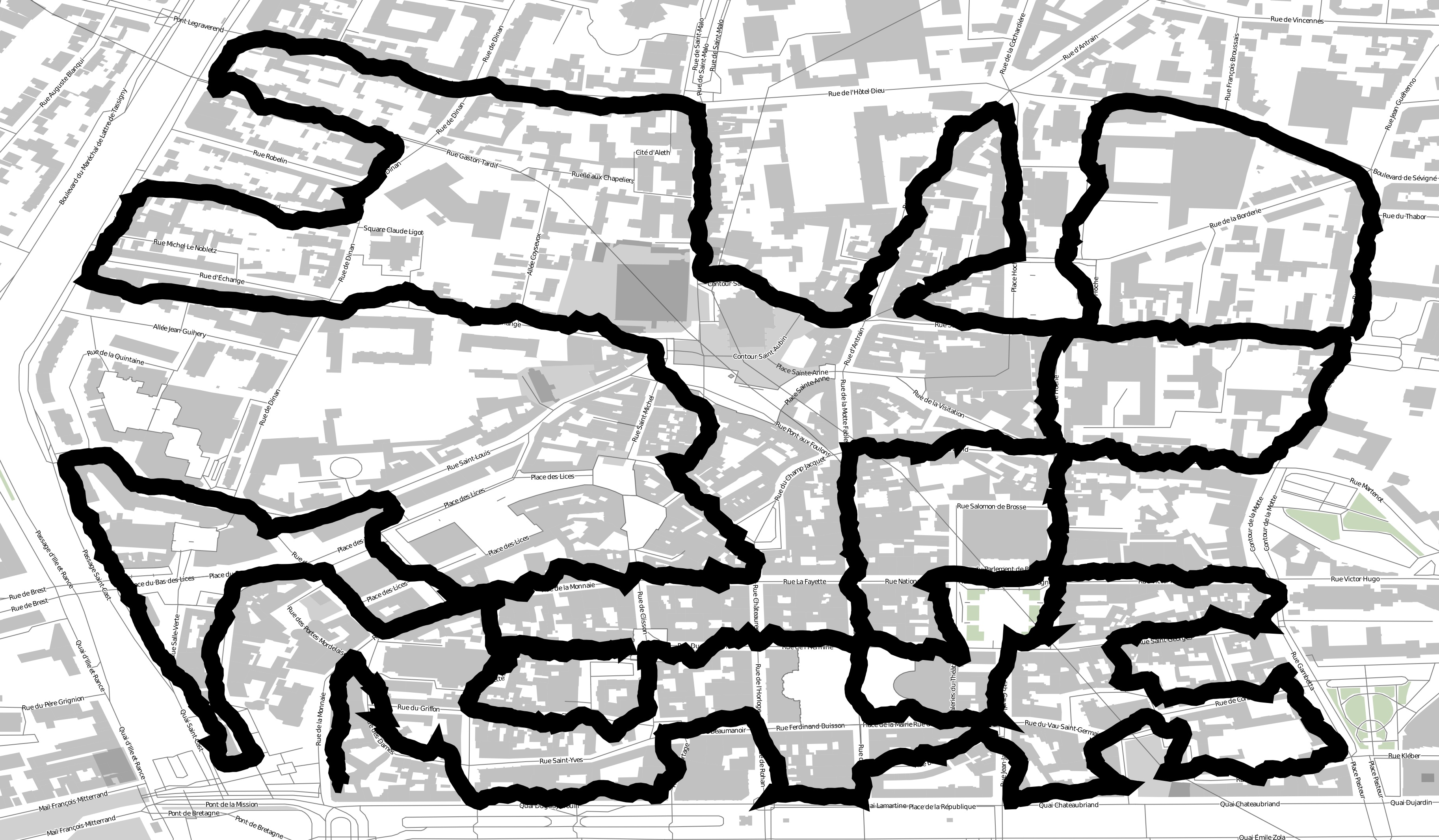
Figure 2(a) : First path : a loop Figure 2(b) : second path: zizag in narrow streets
We walked for more than 20 hours in the center of Rennes (France) (see Figure 2) carrying smartphones running the Wi2Me application [14] (“war-walking”). This application scans periodically all the WiFi channels and logs all the available APs, generating a set of Wi2Me Traces, containing the time, the GPS location and other information about the discovered AP. We then process one or more of these traces to produce a Coverage Matrix, as presented in Figure 3. The Coverage Matrix is a representation of the AP availability: each AP is presented in a column, while we have each scanning event in rows. A black box (or a binary one) means that an AP has been seen during the given scanning event. We can see that AP coverage is usually not continuous: we observe alternative white and black areas for some APs. Some of these gaps are due to link error during the scanning process, while others are simply obstacles that avoid a mobile terminal to correctly receive the AP signal at certain locations in a street.
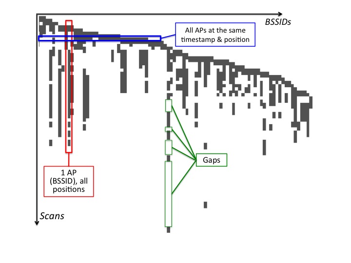
Figure 3: The coverage matrix, which reprense the AP availabilities along a path
In these experiments, we discovered around 8000 APs, and 17 APs per scanning, which reveal a really dense deployment.
Proposed algorithms
Our goal is to evaluate how many AP could be enough to cover the studied areas. Clearly, there is no need for so many APs to cover the path: a mobile terminal can be currently served by 17 different APs at any location on the map. We proposed two algorithms to compute what we call the minimal AP sets.
Algorithm 1: The greedy
- Calculate the total coverage value for the APs, i.e., the sum of all the ones in the corresponding column of the Input Matrix.
- Select the AP with the largest total coverage value and add it to the Minimum APs Set.
- Delete the lines where there is a one in the column of the selected AP from the Input Matrix.
- Delete the column of the selected AP from the Input Matrix.
- Go to Step 1 and repeat until all the lines are deleted.
Algorithm 2: The continuous Greedy
- Starting from the beginning of the path, i.e., the first line of the Input Matrix, identify the available APs (the columns where there are ones in this line).
- Calculate for each of these APs the continu- ous coverage (sum of successive ones starting from the current position until the first zero).
- Choose the AP with the longest continuous coverage and add it to the Minimum APs Set.
- Go to the last line of the continuous coverage of the selected AP.
- Repeat steps 2 to 4 until the end of the matrix i.e end of the path.
Main results
After applying the algorithm, we found that around 6.5% of the detected APs are sufficient to provide full coverage of the path. This percentage varies from 4.25% to 10.91% depending on the dataset, the phone, and the AP selection algorithm. In other words, we can maintain the coverage of a path while switching off at least 89% of the existing APs. This means that the potential of energy saving obtained by switching off the non selected APs is about 89% too. We estimated the energy consumed by the selected APs using the results of [17], which reported that the average consumption of a single AP is about 6 W. Results show that the selected APs consume around 540 W in average for the Loop path and 1215 W for the Zigzag path. This reflects a significant reduction in energy consumption when compared to the initial estimated consumption of 7200 W and 19 323 W for the two paths respectively.
Results also show that the minimal AP set offers a good overlapping. The number of APs seen at any position of the path varies between 1 and 6, with a mean of approximately 2, and an overlapping of two or more APs along more than 60% of the path. Compared to the initial situation where we had an average of 17 APs present at each position of the path, this represents a large reduction in overlapping. The overlapping in the minimal set is useful to insure smoother handovers.
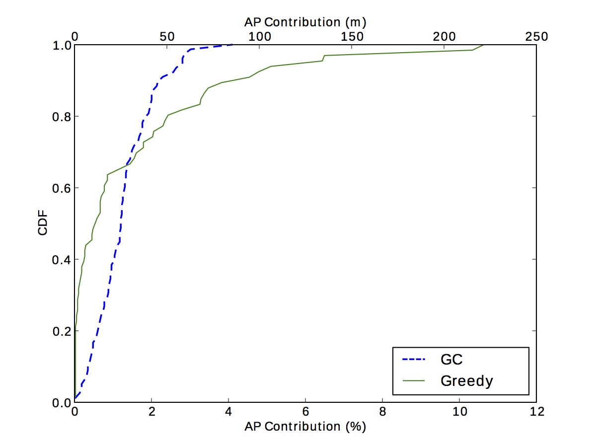
Figure 4: Coverage of the minimal AP sets
Finally Figure 4 shows the contribution of each AP from the minimal AP set. By contribution, we mean the coverage that each of these APs provide to the user. We can see that there is a large portion of the set that does not provide a large coverage: with the greedy algorithm, 75% of the APs are contributing for less than 2% of the total coverage of the path, and we observed that using only the 60% of the *best* AP still provides 98% of path coverage.