Closed-loop stability analysis

Contents

Pisa is a toolbox for closed-loop stability analysis. On this page, we explain how a closed loop stability analysis works and how to set up simulations on electronic circuits to perform such a stability analysis.

After you obtained the correct frequency response function of your circuit, the Pisa tools can kick into action. First, you will project the frequency response onto unstable basis functions to determine whether it is stable or not. When you detect an instability, you can estimate the location of the unstable poles.

Closed-loop stability analysis

Suppose we have a linear system $H$ placed in a feedback configuration as shown below:

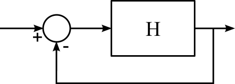
We now want to determine whether this closed-loop system is stable or not.

In a classical open-loop stability analysis, we would analyse the frequency response of $H$ to determine the stability of its closed-loop counterpart. Classical open-loop stability analysis tools include plotting the Nyquist diagram of the loop gain and determining its gain and phase margins.

The open-loop techniques work nicely when the system under test is Single-Input Single-Output (SISO). Applying open-loop methods becomes more difficult in systems built with Multiple-Input Multiple-Output blocks with many different feedback loops. Electronic circuits, especially high-frequency circuits, the circuit components cannot be modelled as SISO blocks due to the reverse gain and non-ideal input and output impedance of the components at high frequencies. This is why closed-loop stability analysis methods have become popular for the stability analysis of high-frequency circuits.

In a closed-loop stability analysis, the frequency response of the closed-loop system is analysed. For this simple system, the closed-loop frequency response is given by:

$\displaystyle G\left(j\omega\right) = \frac{H\left(j\omega\right)}{1+H\left(j\omega\right)} \qquad \mathrm{or} \qquad G\left(j\omega\right) = \frac{1}{1+H\left(j\omega\right)}$

For a realistic system, the closed-loop system is unstable when its closed-loop transfer function $G$ has poles in the complex right half-plane. A closed-loop stability analysis therefore boils down to determining whether a given $G$ has poles in the right half-plane. The pisa toolbox contains the tools to determine whether a given frequency response has poles in the right half-plane. We use projection to determine whether the frequency response has poles in the right half-plane. When an instability is detected, the location of the unstable poles is estimated.

Note that the two closed-loop transfer functions shown above have the denominator and therefore the same poles. This property is valid for any closed-loop frequency response.

All possible closed-loop transfer functions of a system have the same denominator.

This common-denominator property is a second strong-point of a closed-loop stability analysis: the location of the analysis is not cirtical. We discuss this point in greater detail in “Choosing the node to excite”

Stability analysis of circuits

In the context of electronic circuits we analyse circuit’s impedance presented to a small-signal current excitation to perform a closed-loop stability analysis. The simulation set-up used to determine the circuit impedance is shown below:

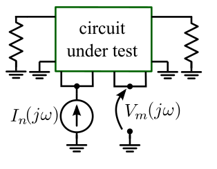
The circuit is terminated in the correct input and output impedances and a small-signal excitation current source is connected to an internal node $n$ of the circuit. The circuit’s resulting voltage response is determined using an AC simulation and measured at node(s) $m$ . The impedance is then computed as:

$\displaystyle Z_{mn} = \frac{V_m\left(j\omega\right)}{I_{n}\left(j\omega\right)}$

To avoid missing an instability, the frequency range of the AC simulation should exceed the bandwidth of all active devices in the circuit. To avoid missing low-frequency instabilities in the biasing networks of amplifiers, make sure to simulate down to 0Hz.

The frequency range should go from 0Hz to beyond the active element’s bandwidth.

Suppose that we have $N_i$ different excitation current sources and $N_v$ measured voltage responses to each current source. All $Z_{mn}$ share a common denominator, so they are best analysed together as a MIMO impedance matrix. To that end, we gather the different impedances and admittances in a matrix

$\displaystyle \mathbf{Z}\left(j\omega\right)=\left[\begin{array}{ccc} Z_{11}\left(j\omega\right) & \cdots & Z_{1N_i}\left(j\omega\right)\\ \vdots & \ddots & \vdots\\ Z_{N_v 1}\left(j\omega\right) & \cdots & Z_{N_v N_i}\left(j\omega\right) \end{array}\right]$

When you have determined your circuit’s impedance, the Pisa toolbox provides the following tools to perform a full stability analysis. First, we project $Z\left(j\omega\right)$ onto a basis for stable and unstable functions to determine its stability. When an instability is detected, we estimate its location.

Analysing the circuit admittance

You can also use small-signal voltage sources to excited the circuit in a closed-loop stability analysis. In that case, the circuit’s admittance is analysed, instead of its impedance. Voltage source excitations should be added in series with a branch of the circuit:

The small-signal voltage source has been added in series with branch $n$ , while its current response is measured at branch $m$ . The circuit admittance function is then defined as:

$\displaystyle Y_{mn}\left(j\omega\right) = \frac{I_m\left(j\omega\right)}{V_{n} \left(j\omega\right)}$

Like in the impedance case, when you have multiple admittances, they can be gathered in an admittance matrix for a common-denominator stability analysis.

Choosing the node to excite

All possible $Z_{mn}\left(j\omega\right)$ and $Y_{mn}\left(j\omega\right)$ in a circuit have the same poles, so the impedance for closed-loop stability analysis can be chosen quite freely. This is one of the advantages of a closed-loop stability analysis.

It can however happen that an unstable pole is hidden by a zero in the denominator. In the literature, this is called a pole-zero cancellation, and it can hide an instability. To avoid pole-zero cancelllations, it is recommended to excite the circuit close to active elements which can cause the instability. Also, when a part of the circuit is symmetric, ensure to break that symmetry, by adding a current excitation to one of the symmetrical parts.

For example, consider the amplifier shown below

Due to the symmetry in this circuit, an odd-mode instability will not be observable when the small-signal perturbation is added at the location of the circuit terminations. In a circuit like this, it is important to add the perturbation source in one to the two branches, to break the symmetry and to be able to detect the possible odd-mode instability.

Circuits with distributed elements

When the circuit contains only lumped elements, like resistors, capacitors and inductors, its frequency response is a rational function. In that case, we could use a rational approximation to find the poles of the circuit and check afterwards whether one of them lies in the right half-plane. For large circuits, the total amount of poles in the circuit becomes very large, which will slow down approaches based on rational approximation.

When distributed elements, like transmission lines, are present in the circuit, the problems get even worse. The transfer functions of distributed circuits are no longer rational, but meromorphic. Detecting the poles of a meromorphic function is a very hard problem because the meromorphic functions can have an infinite amount of poles.

That is why pisa does not use an approach based on approximation, but why we use projection instead. By projecting the impedance onto a basis of stable and unstable functions, we can detect unstable poles without the need of computing a rational approximation of the system. For more information about our projection-based approach, refer to the projection page.

Realistic circuits

When all passives in a circuit are lossy and all active elements have a finite bandwidth, we call a circuit realistic. One can prove that a realistic circuit can only have a finite number of unstable poles. When a realistic circuit contains transmission lines, it will therefore have an infinite amount of stable poles but only a finite amount of unstable poles.

A realistic circuit can have only a finite amount of unstable poles.

When using a projection onto stable and unstable basis functions, we can exploit this fact nicely. The projection allows us to split the frequency response function into a stable part (which has all the stable poles) and an unstable part (which has the unstable poles).
In a realistic circuit, the unstable part only has a finite amount of poles, it is therefore a rational function. In the pisa toolbox, we therefore include a rational approximation method to allow estimating the location of the unstable poles.

The stable part can have an infinite amount of poles and remains meromorphic, so we cannot determine the pole location exactly.

Analysis of a Large-Signal orbit

In a large-signal stability analysis, the stability of a large-signal solution of the circuit is investigated. The circuit is driven by a periodic continuous-wave excitation at a pulsation $\omega_{ex}$ and the circuit solution is obtained with a Harmonic Balance (HB) simulation. Because HB imposes a frequency grid before looking for a solution, it is possible that the obtained solution is not stable. A stability analysis is needed!

Just like in the small-signal case, we add a small-signal perturbation to the obtained circuit solution and analyse the obtained frequency response. When this frequency response has poles in the complex right half-plane, the HB solution is unstable. In case we use a small-signal current excitation, we obtain the following simulation set-up:

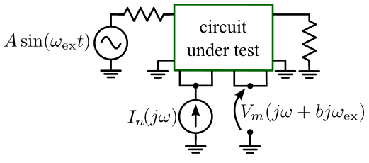
The frequency response of the linearised system around the HB orbit is obtained with a mixer-like simulation (In Keysight’s Advanced Design System (ADS), this mixer-like simulation is called a Large-Signal Small-Signal (LSSS) analysis). As the small-signal will mix with the large signal, several transfer impedances with a different frequency translation are obtained:

$\displaystyle Z_{mn}^{\left[ k \right]}\left(j\omega\right) = \frac{V_m\left(j\omega + jk\omega_{ex}\right)}{I_n\left(j\omega\right)}$

In the literature on linear time-periodic systems, this frequency response function with frequency translation is called a Harmonic Transfer Function (HTF). All HTFs have the same poles, so they should be analysed like a MIMO system. To that end, we gather several HTFs in a vector:

$\displaystyle \mathbf{Z}_{mn}\left(j\omega\right)=\left[\begin{array}{c} \vdots \\ Z_{mn}^{[-1]}\left(j\omega\right) \\ Z_{mn}^{[0]}\left(j\omega\right) \\ Z_{mn}^{[1]}\left(j\omega\right) \\ \vdots \end{array}\right]$

The amount of HTFs to add to this vector depends on the simulation accuracy. In the examples, we show that using HTFs -2 to +2 yields clear results. When several voltages are measured and several small-signal current sources are applies, different HTF vectors can be combined into a large matrix just as in the small-signal case.

Once the different HTFs have been gathered, their stability analysis is no different from the small-signal case. Just use PisaProject to determine the stability of the circuit solution.

Poles in large-signal impedances

When an instability is detected in the large-signal solution using the projection method, we can try to recover the location of the unstable poles, just like in the small-signal case. For a large-signal solution, this is a lot more difficult however.

Theory learns us that the HTFs of the periodic solution of a lumped circuit are given by:

$\displaystyle Z_{mn}^{[l]}(s) = \sum_{p=1}^{N} \sum_{c=-\infty}^{+\infty} \frac{R_{p,c}}{s-{a_p-cj\omega_{ex}}}$

where $N$ is the order of the system. $R_{p,c}$ is the residues of each pole, and $a_p$ are the base poles in the model. The location of these base poles is linked to the Floquet exponents of the periodic system.

The HTFs are clearly not rational functions, due to their infinite amount of poles. When there is an unstable base pole in the system, an infinite amount of copies will also be present in the right half-plane. The unstable part will therefore not be rational and it will be more difficult to estimate the exact pole location.

Non-Hermitian HTFs

The mixer-like simulation in ADS uses Single-Sideband (SSB) current excitations $i(t) = e^{j\omega t}$ , which causes the obtained frequency responses $Z_{mn}^{\prime \left[ k \right]}$ with $k \neq 0$ to be non-Hermitian:

$\displaystyle Z_{mn}^{\prime\left[k\right]}\left(j\omega\right)\neq\overline{Z_{mn}^{\prime\left[k\right]}\left(-j\omega\right)}$

An alternative representation can make $Z_{mn}^{\prime\left[k\right]}$ Hermitian by transferring to a sine and cosine basis from the exponential basis

$\displaystyle Z_{mn}^{\prime\left[k\right]}\left(j\omega\right) =\frac{1}{2}\left[Z_{mn}^{\prime\left[b\right]}\left(j\omega\right)+Z_{mn}^{\prime\left[-b\right]}\left(j\omega\right)\right]$
$\displaystyle Z_{mn}^{\prime\left[-k\right]}\left(j\omega\right) =\frac{j}{2}\left[Z_{mn}^{\prime\left[b\right]}\left(j\omega\right)-Z_{mn}^{\prime\left[-b\right]}\left(j\omega\right)\right]$

References

A. Suarez and R. Quere, Stability analysis of nonlinear microwave circuits. Artech House, 2002.

A. Suarez, “Check the stability: Stability analysis methods for microwave circuits,” Microwave Magazine, IEEE, vol. 16, no. 5, pp. 69–90, June 2015.