Balanced Amplifier

Contents

In this example, we analyse the stability of a balanced amplifier built for operation at 3.6GHz. BFP520 transistors were used to construct the ampliﬁer. During measurement, the design oscillated around 1.43 GHz when terminated with 50Ω. So we should find the same instability using the Pisa analyisis tools.
The amplifier was designed as part of a student project by Kurt Homans and Johan Nguyen.

Simulation set-up

We use the ADS schematic shown below:

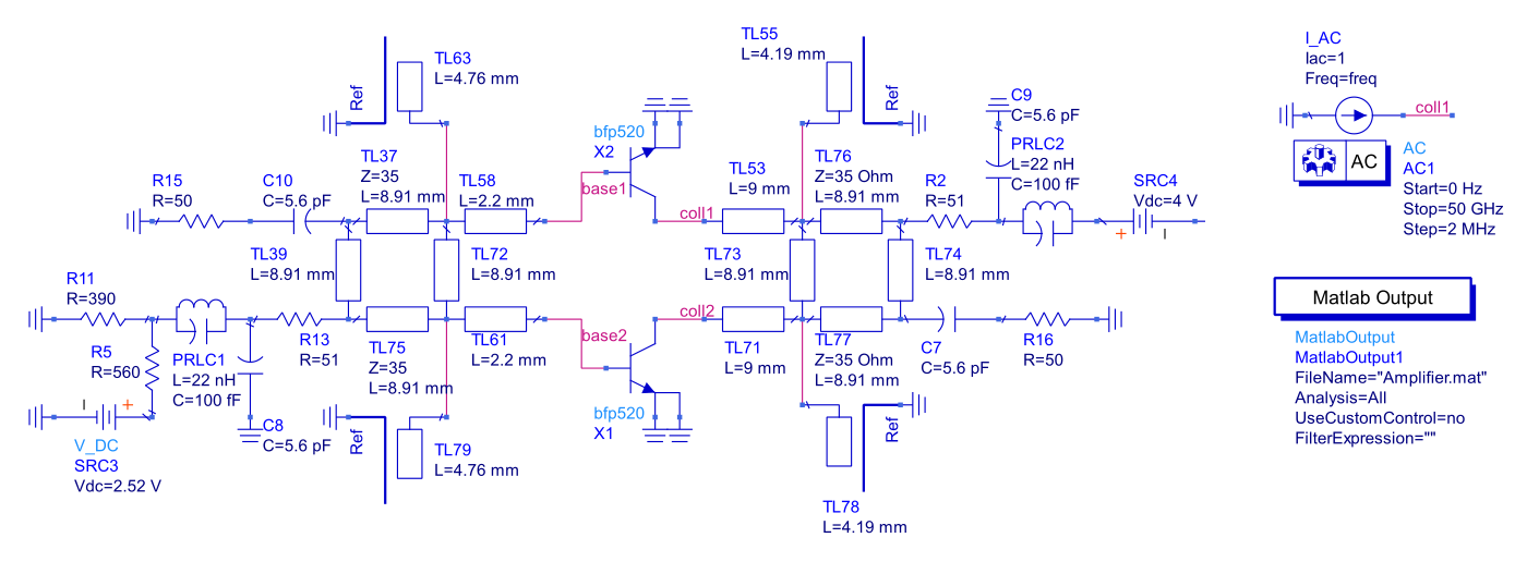
All transmission lines in the circuit are 50Ω lines unless stated otherwise. The TLINP model was used for the transmission lines with $\varepsilon_r = 6.15$ , $\tan(\delta) = 0.003$ and conductor losses $A = 2.5 \frac{\mathrm{dB}}{\mathrm{m}}$ .

We wish to study the stability of the DC solution of this circuit, so we connect a small-signal current source to the collector of the top transistor and run an AC simulation to determine the circuit’s voltage response to the perturbation. We measure 4 voltages in the circuit: at the base and collector of the two transistors.

The BFP520 has an $f_t$ of 45GHz, so we run the AC simulation from 0-50GHz, to cover the complete frequency interval in which an instability can occur. To obtain a sufficiently fine frequency grid, we choose a frequency step of 2MHz.

With a MatlabOutput block, we save the simulation results to a mat file to be imported into Matlab for analysis. When no fixed path is specified, ADS will save this mat file in the data folder of the workspace.

Import into Matlab

To import the simulation data into matlab, we use the ADSimportSimData fuction on the mat file generated by ADS:

1	simdata = ADSimportSimData('Amplifier.mat');

simdata is now a matlab struct with one field: “sim1_AC”, which contains the simulation results of the AC simulation. “simdata.sim1_AC” is a struct with the measured AC voltage responses to the small-signal current source and a frequency axis. following fields:
base2: [1×25001 double] coll2: [1×25001 double] base1: [1×25001 double] coll1: [1×25001 double] freq: [1×25001 double]

We want to analyse the circuit impedance

$\displaystyle Z_i = \frac{V_i}{I_{ex}}$

$I_{ex}=1$ because we excited the circuit with a small-signal current source of 1A. We have $Z_i = V_i$ and we can just analyse the voltage response with the Pisa tools. First, we analyse only the impedance at the excited node. To this end, we gather the data measured at the collector of the top transistor and the corresponding frequency axis. Both are then used to construct an FRM object:

data = reshape(simdata.sim1_AC.coll1,1,1,[]);
freq = simdata.sim1_AC.freq;
% construct the FRM
Z = FRM(data,'Freq',freq,'Normalisation',LowpassNormalisation(freq));

Note that we use a lowpass normalisation in the FRM object. We can do this because we have the impedance information at DC.

Projection

We are now ready to compute the projection on stable and unstable basis functions. To obtain good interpolation results in the sharp resonances in our impedance data, we use a rational interpolation method.

6	PROJ = PisaProject(Z,'Interpolation',RationalInterpolation);

We plot the results of the projection.

figure(1)
plot(    Z        ,'Color',[0 0.4 0],'linewidth',2);
plot(PROJ.stable  ,'Color','b','linewidth',2);
plot(PROJ.unstable,'Color','r','linewidth',2);
xlim([0 max(Z.Freq)])
ylim([-20 60])
legend('original data','stable part','unstable part')

The result is the following:

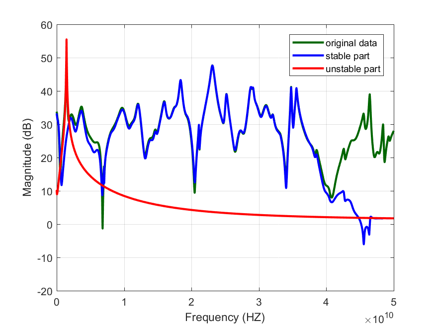
The system is clearly unstable, with an unstable pole around 1.4GHz. We will use PisaEstimate later to determine the exact pole location. Note that the unstable part of the impedance is very simple compared to the complex dynamics present in the stable part. This is a big advantage of working with a projection. Because all passives used in the simulation set-up are lossy and because the transistor has a finite bandwidth, we know that the stable part is rational. All distributed effects due to the transmission lines in the circuit appear in the stable part of the projection.

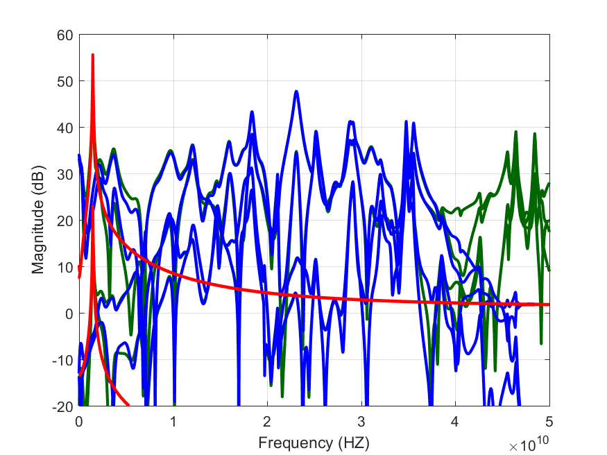
It is just as easy to run the projection on all impedance traces at the same time. Now, instead of adding only the voltage at the first collector to the data in the FRM, we add all 4 of the measured impedances in the FRM, such that the system we analyse becomes a 1-input 4-output system. The rest of the code remains unchanged:

data = [simdata.sim1_AC.coll1;
        simdata.sim1_AC.coll2;
        simdata.sim1_AC.base1;
        simdata.sim1_AC.base2];
freq = simdata.sim1_AC.freq;
% gather the data and frequency in an FRM
Z = FRM(reshape(data,4,1,[]),'Freq',freq,'Normalisation',LowpassNormalisation(freq));
% call the projection method
PROJ = PisaProject(Z,'Interpolation',RationalInterpolation);
% plot the result
figure(2)
plot(    Z        ,'Color',[0 0.4 0],'linewidth',2);
plot(PROJ.stable  ,'Color','b','linewidth',2);
plot(PROJ.unstable,'Color','r','linewidth',2);
xlim([0 max(Z.Freq)])
ylim([-20 60])

The result is a little bit more confusing to analyse, but the instability is clearly visible in all impedance functions:

Estimation

We now use the results of the projection of the 1-input 4-output frequency response to determine its common poles. We estimate the pole location with the help of the PisaEstimate function

poles = PisaEstimate(Z,'Projection',PROJ);

Because we don’t provide the order of the unstable part of the system, the function will show the singular values of the Hankel matrix to allow the user to specify the order. For this example, we obtain the following singular values:

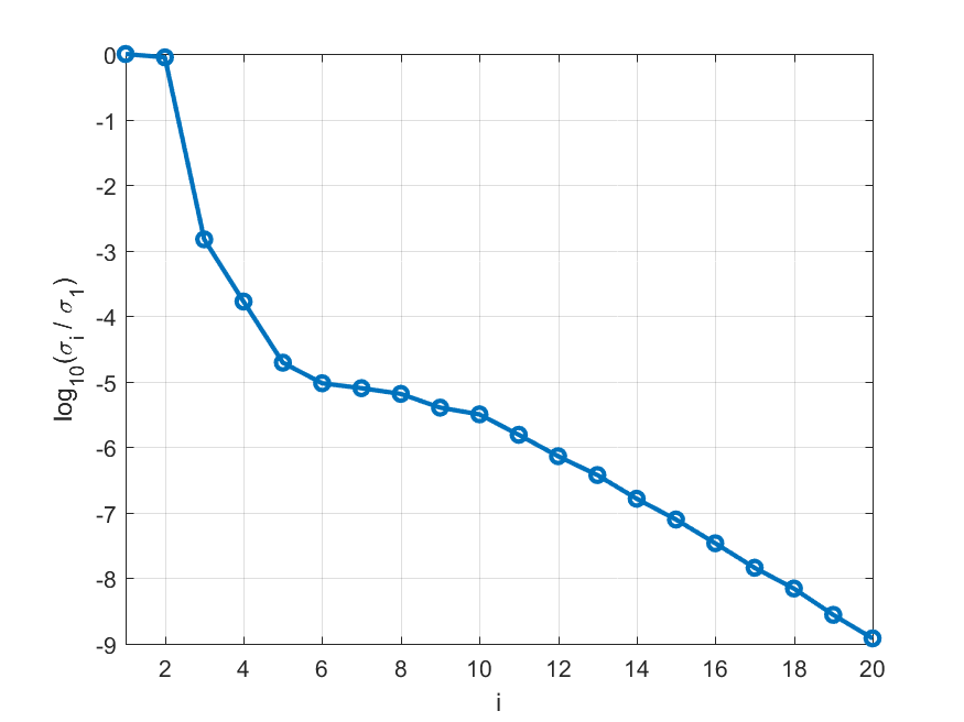
There are two significant singular values, so the amplifier has two unstable poles (A complex-conjugate resonant pole pair). We give 2 as order of the system and obtain the following result:

fprintf('poles estimated at: %g GHz\n',abs(imag(poles(1)))/2/pi/1e9);
fprintf(' with a damping of %2.2g \n',cos(pi-angle(poles(1))));

poles estimated at: 1.45979 GHz with a damping of -0.014

Download code and workspace

Click here to download the ADS workspace with all the examples and the matlab code to run pisa.