Large-signal stability analysis

Contents

In this example, we show how pisa can be used to perform a large-signal stability analysis. In the page on closed-loop stability analysis, we explained that the stability of a large-signal orbit can be determined in the same way as the stability of a small-signal orbit: compute the frequency response of the circuit when linearised around the orbit and determine whether that frequency response has poles in the complex right half-plane.

The approach we follow is therefore the same as with the small-signal examples. We first determine the frequency response. Then we project the frequency response ont stable and unstable basis functions to determine whether an instability is present. When we find an instability, we estimate the location of the unstable poles. Estimating the poles is more complicated here, because theory predicts that the unstable part will not have a finite amount of poles in the right half-plane.

The circuit we analyse here is very simple, it consists of a series connection of a resistor, inductor and a diode.

The diode has a non-zero transit time $\tau$ which causes the chaotic eﬀects in the circuit.

This circuit is known to generate period-doubling solutions starting from a certain input amplitude. It is therefore a good candidate for a large-signal stability analysis. To visualise the circuit behaviour, I used a transient simulation. I simulated 1000 periods of the input source and used only the ﬁnal 30 for further analysis.
I created a Poincaré diagram of the current to visualise the circuit behaviour. To do so, I sample a single point in the steady-state current time-domain waveform every $(100 \mathrm{kHz})^{-1}$ , which is the period of the generator. When a single point is obtained in the Poincaré diagram, the current has the same period as the input generator.

When two points appear, a period-doubling has occurred in the circuit and the current has
For low amplitudes of the input voltage $V_\mathrm{in}$ , the circuit acts normal. Starting from $0.8V$ , a period-doubling is observed. Above $1.7V$ the period of the current is four times the input period. At the highest voltages, chaos is observed. When Harmonic Balance (HB) is used to determine the solution of this circuit, it can ﬁnd the unstable solutions of the circuit (indicated with the grey lines in the Poincaré plot).

Projection at 0.5V drive level

We start by importing the simulation data from the mat file generated by ADS:

1	simdata = ADSimportSimData('LargeSignal_0.5V.mat');

simdata is now a struct with two fields: “sim1_HB” contains the results of the Harmonic Balance simulation and “sim2_LSSS” contains the results of the Large-Signal Small-Signal simulation performed around the obtained HB solution. “sim2_LSSS” is a struct with the following fields:

freq: [2001×21 double] Vd: [2001×21 double] I_SRC1: [2001×21 double] sweepvar_ssfreq: [2001×1 double] Mix1: [2001×21 double] Mix2: [2001×21 double]

These results are difficult to work with, so we provide a function to extract the Harmonic Transfer Functions (HTF) from the LSSS data. To ensure that the HTFs at negative frequencies is the conjugate of the data at positive frequencies, we work with a sine and cosine basis for the HTFs.

2	HTFdata=LSSSextractHTFs(simdata.sim2_LSSS,'Basis','cosine');

HTFdata is a matlab struct with the following fields:

freq: [2001×1 double] Vd: [21×2001 double] I_SRC1: [21×2001 double]

where “freq” is the frequency axis and “Vd” contains 21 HTFs: $Z_{-10}$ to $Z_{+10}$ .

We gather $Z_{-2}$ to $Z_{+2}$ is a 1-input 5-output FRM:

3
4
5

freq = HTFdata.freq;
data = reshape(HTFdata.Vd((end-1)/2+1+(-2:2),:),5,1,[]);
Z_lowamp = FRM(data,'Freq',freq,'Normalisation',LowpassNormalisation(freq));

We cannot simulate at exactly 0Hz, due to the limitations of the Large-Signal Small-Signal simulation of ADS, but we get sufficiently close to allow a good prediction of the circuit behaviour at DC.

5 6	Z_lowamp = FRM(data,'Freq',freq,'Normalisation',LowpassNormalisation(freq)); PROJ_lowamp = PisaProject(Z_lowamp,'EstimateInterpolationError',true);

Because we are using a lowpass normalisation without impedance information at 0Hz, the projection function will return the following warning:

Warning: No DC value was provided. The DC value will be predicted using extrapolation, which might introduce errors

But we will ignore this warning here, because we know that the predicted value at 0Hz will be accurate.

We plot the results:

figure
plot(Z_lowamp,'Scale','Hz','Color','g');
plot(PROJ_lowamp.unstable,'Scale','Hz','Color','r');
plot(PROJ_lowamp.stable ,'Scale','Hz','Color','b');
plot(PROJ_lowamp.InterpErr ,'Scale','Hz','Color','k');
xlim([0 max(Z_lowamp.Freq)]);
ylim([-100 100])

The unstable part of the HTFs is very low, and for most of the frequencies, it lies below the estimated interpolation error. At the high-frequency side, you can see some influence of the end of the simulation interval, which is not fully suppressed by the analysis filter.

Stability analysis at 1.5V drive level

We run exactly the same code, but now with the high amplitude data.

simdata = ADSimportSimData('LargeSignal_1.5V.mat');
% extract the Harmonic transfer functions from the imported simulation data
HTFdata=LSSSextractHTFs(simdata.sim2_LSSS,'Basis','cosine');
freq = HTFdata.freq;
data = reshape(HTFdata.Vd((end-1)/2+1+(-2:2),:),5,1,[]);
% create the FRM and project
Z_highamp = FRM(data,'Freq',freq,'Normalisation',LowpassNormalisation(freq));
PROJ_highamp = PisaProject(Z_highamp,'EstimateInterpolationError',true);
% show the result
figure
plot(Z_highamp,'Scale','Hz','Color',[0 0.4 0],'linewidth',2);
plot(PROJ_highamp.unstable,'Scale','Hz','Color','r','linewidth',2);
plot(PROJ_highamp.stable  ,'Scale','Hz','Color','b','linewidth',2);
% plot(PROJ_highamp.InterpErr ,'Scale','Hz','Color','k','linewidth',1);
xlim([0 0.6e6]);
ylim([30 90])

Here the solution is clearly unstable:

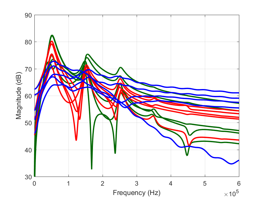
It is interesting to note here that the unstable part peaks at $50\mathrm{kHz}+k\cdot 100\mathrm{kHz}$ , which are the frequencies the circuit wants to generate to go to its period-doubling stable solution.

Pole estimation at the 1.5V drive level

In the analysis of a large-signal solution, the amount of unstable poles is theoretically infinite, due to the fact that each unstable Floquet multiplier causes an infinite chain of poles on a vertical line in the complex plane. In theory, it will therefore be impossible to obtain a perfect rational approximation of the unstable part of an HTF.

In the unstable part we observe here though, we notice that the higher-order copies of the main pole are not really visible in the data, so we can try our approximation routine to see what it returns:

[poles,singularvalues] = PisaEstimate(Z_highamp,'Projection',PROJ_highamp);

Because we don’t specify the amount of unstable poles we are looking for, the function will show the singular values and ask for the order. The singular values look like this:

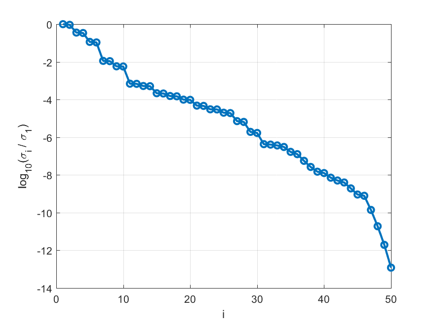
There is no clear jump in the singular values now. This is to be expected, due to the fact that the unstable part of an HTF has an infinite amount of copies of the base pole. We choose order 10 for lack of a better choice:

Enter the amount of unstable poles: 10

And we plot the obtained poles in the complex plane. We divide by $2\pi$ because we want to see the frequency of the poles, not the pulsation:

figure
plot(poles/2/pi,'x','linewidth',2);
grid on
xlim([0 2*max(real(poles/2/pi))])
xlabel('Real part [Hz]')
ylabel('Imaginary part [Hz]')

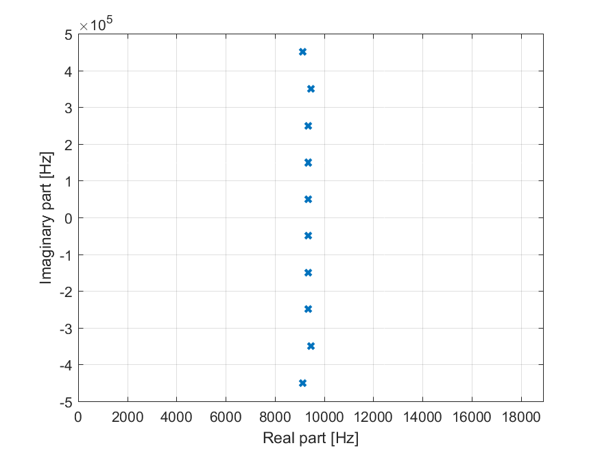
The first few copies of the poles are nicely spaced on a vertical line, which is what theory predicts. The higher-order copies are not so well estimated and stray from their theoretical spot.

Download code and workspace

Click here to download the ADS workspace with all the examples and the matlab code to run pisa.