Oscillator – PISA

Contents

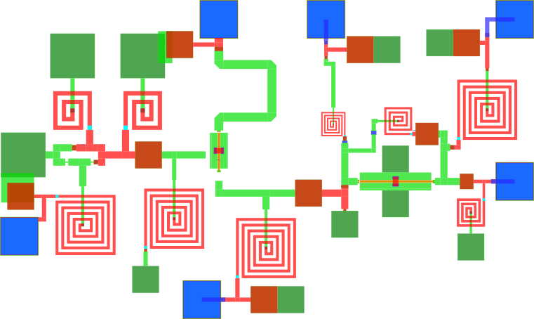
In these several examples, we will analyse the stability of the following MMIC oscillator from the example library of ADS:

Most of the transmission lines in the design are modelled using MLIN components. The inductors and capacitors are taken from the DemoKit library. To determine the behaviour of the meandering transmission line above the first transistor, a Momentum simulation is used.

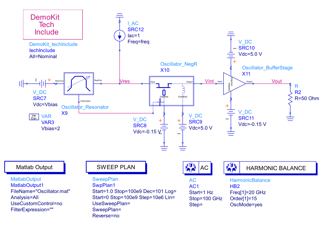
To determine the circuit impedance, we connect a small-signal current source between the resonator and the oscillating transistor. With an AC simulation, we determine the resulting voltage at two nodes: $V_{int}$ and $V_{out}$ .

The simulation set-up is shown below:

Importing the simulation data

We start by loading the simulation data:

1	simdata = ADSimportSimData('Oscillator.mat');

simdata is now a matlab struct that contains the following fields: one field (sim1_AC) contains a struct with the AC simulation data, and a second field (sim2_HB) contains a struct for the HB data. We are interested in determining the unstable poles of the DC operating point, so we focus on the AC simulation data. simdata.sim1_AC contains the following fields:

simdata.sim1_AC.Vres: [1×11112 double] simdata.sim1_AC.Vint: [1×11112 double] simdata.sim1_AC.Vout: [1×11112 double] simdata.sim1_AC.freq: [1×11112 double]

To determine the stability of the system, we analyse its impedance:

$\displaystyle Z_m = \frac{V_m}{I_{ex}}$

Because $I_{ex}=1$ in our simulations, we have $Z_m = V_m$ and we can immediately analyse the measured voltages to determine the unstable poles. We gather the three measured voltages into a 1-input 3-output FRM object:

data = [simdata.sim1_AC.Vint;
        simdata.sim1_AC.Vout;
        simdata.sim1_AC.Vres];
freq = simdata.sim1_AC.freq;
Z = FRM(Zdata,'Freq',freq,'Normalisation',LowpassNormalisation(freq));

Project

To check whether the circuit is unstable, we use the Project function:

6	PROJ = PisaProject(Z);

We obtain the following results for the stable and unstable parts:

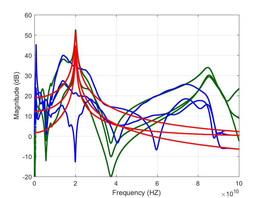
The data is clearly unstable, with a nice unstable resonance around 20GHz.

Estimate

To get a better estimate of the eventual oscillation frequency and of the start-up speed of the oscillator, we want to know the location of the unstable pole.

To do this, we use the PisaEstimate function. To avoid computing the projection twice, we pass the result of our projection to as the “Projection” parameter to the PisaEstimate function.

7	poles = PisaEstimate(Z,'Projection',PROJ)

We don’t know the amount of unstable poles in the system yet, so we don’t specify an order to PisaEstimate. The function will then show a plot of the singular values of the Hankel matrix and ask for the order. In this case, we get the following singular values:

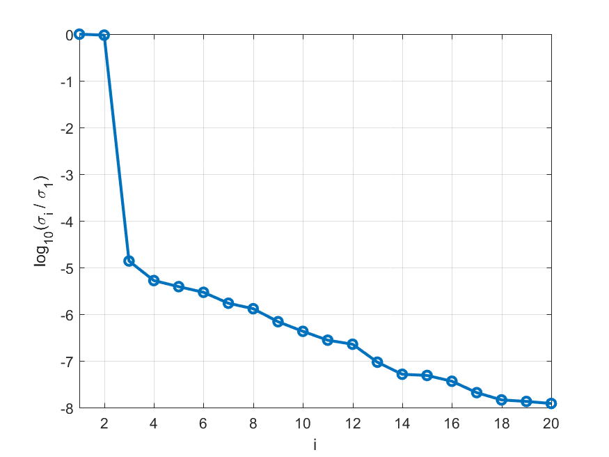
There are clearly two dominant singular values, which indicates that there are two (complex-conjugate) unstable poles in the circuit. We provide order 2 to PisaEstimate and obtain the following poles

7 8	fprintf('poles estimated at: %g GHz\n',abs(imag(poles(1)))/2/pi/1e9); fprintf(' with a damping of %2.2g \n',cos(pi-angle(poles(1))));

poles estimated at: 20.1575 GHz with a damping of -0.014

Download code and workspace

Click here to download the ADS workspace with the examples together and the matlab code to run pisa.