Project – PISA

Contents

On this page, we explain the details and implementation of the PisaProject function. This method of functional projection to perform stability analysis is the foundation of the pisa toolbox.

The concept is simple: to determine the stability of a system, project its frequency response on a basis of stable and unstable functions. when a significant part if projected onto the unstable basis functions, we have detected an instability.

Here, we consider the abstract notion of frequency response of a system. In the stability analysis of a circuit, this frequency response is either the impedance or admittance presented by the circuit to a small-signal excitation source. More information about the simulation set-up required to determine such frequency response can be found on the page on closed loop stability analysis.

If you want to see the functional projection technique applied to several examples, go to the examples page.

Theory

We are given a frequency response matrix $Z\left(j\omega_k\right)$ of a system with $N_o$ outputs and $N_i$ inputs on a discrete set of frequencies $\omega_k$ . We assume that $Z\left(j\omega_k\right)\in \mathcal{L}_2$ , which means that we can write $Z\left(j\omega\right)$ as the sum of a function in the Hardy space $H_2$ (the stable part) and its orthogonal complement $\bar{H}_2$ (the unstable part):

$\displaystyle Z\left(j\omega\right) = Z^\mathrm{stable}\left(j\omega\right) + Z^\mathrm{unstable}\left(j\omega\right)\qquad\mathrm{with}\quad Z^\mathrm{stable}\in H_2 \quad Z^\mathrm{unstable}\in \bar{H}_2$

Computing the stable and unstable parts of a given frequency response is done by projecting onto the basis of $H_2$ and $\bar{H}_2$ respectively:

$\displaystyle Z^\mathrm{stable}\left(j\omega\right) = P_{H_2}\left\{ Z\left(j\omega\right) \right\} \qquad Z^\mathrm{unstable}\left(j\omega\right) = P_{\bar{H}_2}\left\{ Z\left(j\omega\right) \right\}$

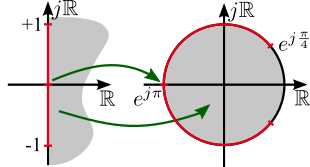
In our algorithm, we map the frequency axis to the unit circle such that the complex right half-plane is mapped to the inside of the circle. After this mapping, $e^{j k \theta}$ with $k >=0$ forms a basis for $H_2$ and $e^{-j k \theta}$ with $k >0$ forms a basis for $\bar{H}_2$ . The projection is therefore performed by computing the Fourier coefficients of our function on the unit circle.

On the unit circle, computing the projection boils down to computing the Fourier coefficients.

The simulated frequency response is only known for frequencies below $f_\mathrm{max}$ . Above that frequency, we assume that the frequency response is zero. This sudden jump to zero at $f_\mathrm{max}$ will have a strong unwanted inﬂuence on the obtained stable and unstable part. To suppress this inﬂuence, the frequency response is multiplied by a low-pass filter with its stop-band starting at $f_\mathrm{max}$ .

Algorithm steps

We can summarise the projection algorithm in the following steps:

Perform a frequency normalisation on $Z\left(j\omega_k\right)$
Transform $Z_\mathrm{norm}\left(j\omega_k\right)$ to the unit circle
Multiply by a filtering function $F\left(\theta\right)$
Compute the Fourier coefficients $f_k$ of $Z_\mathrm{disc}\left(\theta\right) F\left(\theta\right)$
Compute the stable and unstable parts by constructing the functions made of positive and negative Fourier coefficients respectively:

$\displaystyle Z^\mathrm{unstable}_\mathrm{disc}\left(\theta\right)=\sum_{k=-1}^{-N} f_{k} e^{j k\theta} \qquad Z^\mathrm{stable}_\mathrm{disc}\left(\theta\right)=\sum_{k=0}^N f_{k} e^{j k\theta}$

Transform $Z_\mathrm{disc}^\mathrm{stable}$ and $Z_\mathrm{disc}^\mathrm{unstable}$ back to the complex plane
Perform a frequency denormalisation of $Z^\mathrm{stable}$ and $Z^\mathrm{unstable}$

Frequency normalisation

Internally, the data frequency response data is mapped to the frequency interval $[-1,1]$ for ease-of-computation. We provide two different ways to perform this mapping:

In a Bandpass normalisation, we start with data on a frequency interval $[f_\mathrm{min},f_\mathrm{max}]$ and map $f_\mathrm{min}\rightarrow -1$ and $f_\mathrm{max} \rightarrow 1$ . The data outside of the interval is assumed to be zero, so using a bandpass normalisation will cause the system to be non-hermitian $Z(f)\neq \overline{Z(-f)}$ .

When a Lowpass normalisation is used, we map $f_{max}\rightarrow 1$ and $-f_{max}\rightarrow -1$ . In the lowpass case, the system is assumed to be Hermitian, so the data for the negative frequencies is taken to be the complex conjugate from the data at the positive frequencies. Lowpass normalisation is best used when you know the frequency response for $f=0$ . Otherwise, the method will perform an interpolation between $-f_\mathrm{min}$ and $f_\mathrm{min}$ to estimate the value at zero. This interpolation can introduce a large error in some cases, you should use a bandpass normalisation then.

Mapping to the unit circle

After the frequency normalisation, we are ready to transform the data to the unit circle. To this end, we use Mobius transform.

$\displaystyle Z_\mathrm{disc}\left( z \right) = Z\left( \alpha \frac{ z+1}{z-1} \right)$

where $\alpha$ is chosen such that the following mapping happens in the transform:

$\begin{array}{lcl} \omega=+1 & \rightarrow & \theta=+{\displaystyle \frac{\pi}{4}}\\ \omega=0 & \rightarrow & \theta=\pi\\ \omega=-1 & \rightarrow & \theta={\displaystyle -\frac{\pi}{4}} \end{array}$
The complex right half-plane is mapped to the inside of the unit circle. We can visualise the transform like this:

Filtering to suppress edge effects

After frequency normalisation and mapping to the unit circle, we know the frequency response $Z_\mathrm{disc}$ on the interval $\theta = [\frac{\pi}{4} , \frac{7\pi}{4}]$ . Outside this interval, we don’t have any data, so we assume it is zero there. This sudden ending of the data will show up in the unstable part, so its influence needs to be suppressed. We do this by multiplying the data by a filtering function $F$ :

$\displaystyle Z^\mathrm{filtered}\left(\theta\right) = F\left(\theta\right)\cdot Z_\mathrm{disc}\left(\theta\right)$

We then compute the projection of $Z^\mathrm{filtered}$ instead of $Z_\mathrm{disc}$ . This filtering will suppress unstable poles close to the interval boundary. It is therefore recommended to simulate the frequency response of the system on a very wide band to minimise the influence of the filtering on the projection result.

The filter we use is a FIR filter:

$\displaystyle F\left(\theta\right) = \sum_{k=0}^{N_f} a_k e^{j k \theta}$

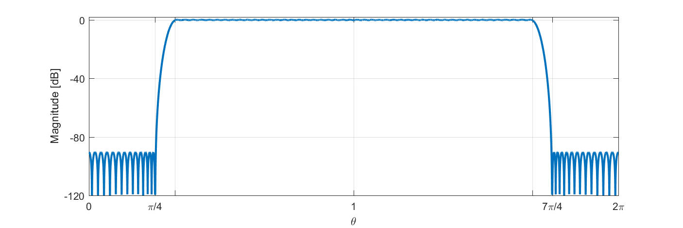
Because it only consists of positive Fourier coefficients, $F$ is stable. Its influence will therefore mainly be visible in the stable part of the projection. The only influence the filter has on the unstable poles it that their residues are modified.

The coefficients of the filtering function are precomputed such that the out-of-band suppresion is maximised, for a fixed in-band ripple and transition region. Also, the filtering function is designed to have no zeros inside of the unit disc. That way, they cannot accidentally coincide with an unstable pole. To enforce smoothness in the derivative of the data at the edge of the interval, Two transmission zeros are placed at $\theta=\frac{\pi}{4}$ .

The default filter we use in PisaProject has order $N_f=76$ , a transistion region of 10% of the data interval and has an in-band ripple of 0.02:

Computing the Fourier coefficients

We provide two different options to compute the Fourier coefficients of the filtered impedance function. The first computes the classic Fourier integral:

$\displaystyle f_k = \int_0^{2\pi} Z_\mathrm{disc}\left(\theta\right) F\left(\theta\right) e^{-j k \theta} d\theta$

using standard numeric integration techniques. The second option uses the Fast Fourier Transform (FFT) to perform the computation.

The number of Fourier coefficients should be large enough to capture the dynamics in the frequency response function. When a sharp resonance is present in the data, a high amount of Fourier coefficients is needed to capture this resonance.

As a small example, consider the unstable resonance shown below:

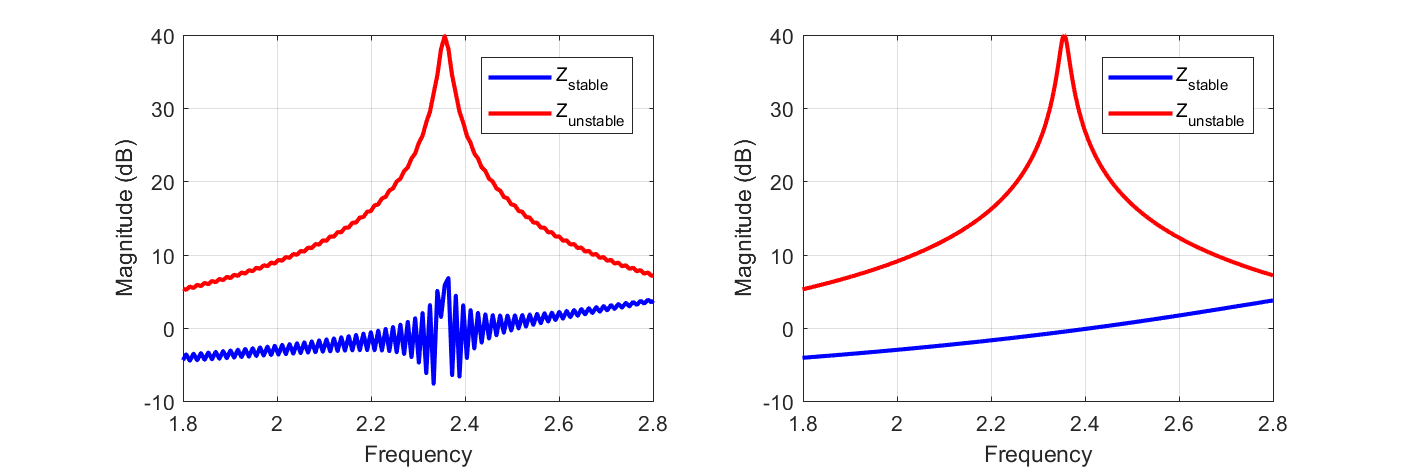
On the left, we used too little Fourier coefficients, which shows oscillations in the stable part around the unstable resonance. When we increase the amount of Fourier coefficients (shown on the right), these resonances disappear.

Choosing the correct amount of Fourier coefficients is not so difficult: more is always better. Performing a trade-off between computation time and accuracy is a little bit more difficult and depends on the data.

Interpolation

Both techniques integration techniques (quadrature and FFT) require to interpolate the function values on the unit circle. We either use a simple linear interpolation method, or a rational interpolation method.

Linear interpolation is the easiest to use and to understand. It should be used when the data is noisy because it does not impose continuous derivatives. When the data contains strong resonances, linear interpolation will perform poorly. This is why we also offer a rational interpolation method. The rational interpolation ensures a continuous first derivative, so it can only be used on noise-free data.

In the rational interpolation scheme, we use a rational interpolation function with two zeros and one pole:

$\displaystyle I_m \left(\theta\right) = \frac{a_m\left(e^{j\theta}\right)^2 + b_m e^{j\theta}+ c_m}{e^{j\theta}+d_m}$

where $a_m$ , $b_m$ , $c_m$ and $d_m$ are determined using the constraints:

$\displaystyle \begin{array}{cc} I_m\left(\theta_{m}\right)=Z_\mathrm{disc}\left(\theta_{m}\right) & I_m\left(\theta_{m+1}\right)=Z_\mathrm{disc}\left(\theta_{m+1}\right)\\ I_m\left(\theta_{m+2}\right)=Z_\mathrm{disc}\left(\theta_{m+2}\right) & \frac{\partial}{\partial\theta}I_m\left(\theta_{m}\right)=\frac{\partial}{\partial\theta}I_{m-1}\left(\theta_{m}\right) \end{array}$

The ﬁnal constraint ensures that the interpolated function has a continuous ﬁrst derivative at the interpolation points.

Estimating the interpolation error

The interpolation introduces both stable and unstable artefacts into the projection method. To estimate the size of these artefacts, we compute an estimate of the interpolation error. The level of this interpolation error can be estimated by interpolating the frequency response using only the data at the even data points. The difference between the original and the interpolated data for the odd data points will give an indication of the interpolation error encountered in the stability analysis.

Interpreting the result

Once the projection has been computed and the impedance function has been split into two parts, we can interpret the results to determine whether the circuit is stable or not. As an example, we show the analysis results for an MMIC power amplifier where a stabilisation resistor is tuned to guarantee circuit stability:

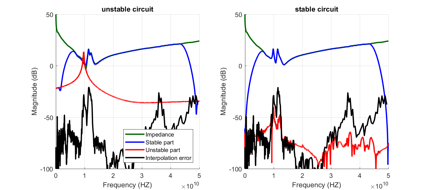
In the plot on the left, the unstable part shows a nice resonance around 10GHz, which indicates an instability. Comparing the size of the obtained unstable part to the level of the interpolation error allows us to affirm that the obtained unstable part is correctly computed and did not arise due to interpolation errors.

In the plot on the right, the unstable part is a lot smaller and more noisy than before. When we compare the unstable part to the interpolation error, we notice that they are both of similar magnitude. This allows us to conclude that the obtained unstable part is due to interpolation errors and not due to an instability in the circuit.

To see more examples on how a result of projection is interpreted, have a look at our different examples.

Implementation

The projection algorithm described above is implemented in the PisaProject function. Before calling that function, we need to store the circuit impedance data in an FRM object:

Z = FRM(data,'Freq',freq);

where data is an $N_o \times N_i \times F$ array which contains the circuit impedance function(s). and freq is the frequency vector of the data (of length $F$ ).

When the data is gathered in the FRM object, we can pass it to the PisaProject function:

PROJ = PisaProject(Z);

The result is a matlab struct with the following fields:

stable: FRM which contains $Z^\mathrm{stable}$
unstable: FRM which contains $Z^\mathrm{unstable}$
coeffs_stable: Positive Fourier coefficients $f_k : k>=0$ (array of size $N_o \times N_i \times N$ )
coeffs_unstable: Negative Fourier coefficients $f_{-k} : k > 0$ (array of size $N_o \times N_i \times N$ )
InterpErr: FRM which contains the estimated interpolation error made during the projection

Setting the normalisation

The frequency normalisation in pisa is a property of the FRM object.

Z = FRM(data,'Freq',freq,'Normalisation',LowpassNormalisation(freq));
PROJ = PisaProject(Z);

Setting the interpolation

The interpolation scheme used in the computation of the Fourier coefficients is controlled by setting the “Interpolation” parameter in PisaProject:

PROJ = PisaProject(Z,'Interpolation',RationalInterpolation);

Where the provided interpolation is an object which implements the abstract Interpolation class. We implemented two different interpolation methods: RationalInterpolation and LinearInterpolation. The default is linear interpolation, because of its speed and robustness.

Linear interpolation performs poorly when sharp resonances are present in the frequency response, a lot of samples are needed inside of the resonance to prevent the interpolation error to become too big. Linear interpolation should be used when the data is noisy because it does not impose a continuous derivative.

The rational interpolation method is perfectly suited for noiseless data with resonances. It is however slower than linear interpolation and it can encounter numerical issues for data which is constant or linear.

Computation of the Fourier coefficients

PisaProject can compute the Fourier coefficients in two different ways: By Fast Fourier Transform, or by quadrature integration. This is controlled by the “Integration” parameter for PisaProject:

PROJ = PisaProject(Z,'Integration','FFT');

The default is to use the FFT because of its speed. It can however introduce aliasing, but it is the best way to compute a large amount of Fourier coefficients. When only a small amount of Fourier coefficients is needed, it is better to use the quadrature integration.

Besides the computation style, one can control the number of Fourier coefficients by setting the “numberOfCoefficients” parameter in PisaProject:

PROJ = PisaProject(Z,'numberOfCoefficients',1e6);

When the FFT is used to compute the Fourier coefficients, setting this parameter correctly is important to avoid aliasing. When the data contains very sharp resonances, a high amount of Fourier coefficients will be needed to avoid this aliasing.

References

A. Cooman, F. Seyfert, M. Olivi, S. Chevillard, and L. Baratchart, “Model-free closed-loop stability analysis: a linear functional approach” IEEE transactions on microwave theory and techniques, vol. 66, no. 1, pp. 73-80, 2018.