Estimate – PISA

Contents

The first step in the pole estimation algorithm is to perform a projection using the PisaProject function. Once the unstable part has been determined, you can estimate the location of the unstable poles with the PisaEstimate function.

Here, we detail the theory and implementation behind the PisaEstimate function. The function estimates the location of the unstable poles in a given frequency function. We assume that you are already familiar with the projection method. If not, please refer first to the projection page.

If you want to see the PisaEstimate function in action, you can check out our list of examples.

Theory

We use the theory introduced by Adamyan, Arov and Krein to recover the location of the unstable poles on the unit disc. It uses the following infinite Hankel matrix which contains the negative Fourier coefficients of $Z_\mathrm{disc}$ :

$\displaystyle \Psi=\left[\begin{array}{ccc} f_{-1} & f_{-2} & \cdots\\ f_{-2} & \ddots\\ \vdots \end{array}\right]$

In practice, we truncate the infinite $\Psi$ to $\Psi=\Psi_{1..N,1..N}$ . $N>50$ has yielded good results in all examples we tried. By Kronecker’s theorem for a rational symbol with $P$ poles, $\Psi_N$ , is of rank $P$ . We compute the rank using the Singular Value Decomposition of $\Psi_N$ . Ideally the number of non-zero singular values of $\Psi_N$ equals the number of poles of the function $Z_\mathrm{disc}^\mathrm{unstable}$ . In practice due to numerical errors, the first $P$ singular values are large when compared to the others. This property is used to determine the number of unstable poles $P$ of $Z_\mathrm{disc}$ .

Principal Hankel Components

Once $P$ has been determined, we can determine the circuit poles using the Principal Hankel Components (PHC) algorithm. Assume we have a state-space realisation of the unstable part of the impendace on the unit circle:

$\displaystyle Z^\mathrm{unstable}_\mathrm{disc} \left(z\right) = C\left(zI-A\right)^{-1}B + D$

The eigenvalues of the $A$ -matrix correspond to the poles of the system. The system’s, observability matrix $\mathcal{O}$ and controllability matrix $\mathcal{C}$ are defined as:

$\displaystyle \mathcal{O} = \left[\begin{array}{c} C\\ CA\\ CA^{2}\\ \vdots \end{array}\right] \qquad \mathcal{C} = \left[\begin{array}{cccc} B & AB & A^{2}B & \cdots\end{array}\right]$

the Hankel matrix is equal to the product of $\mathcal{O}$ and $\mathcal{C}$ :

$\displaystyle \Psi=\left[\begin{array}{cccc} CB & CAB & CA^{2}B & \cdots\\ CAB & CA^{2}B & \ddots\\ CA^{2}B & \ddots\\ \vdots \end{array}\right] =\mathcal{O}\mathcal{C}$

Using the singular value decomposition of the truncated Hankel matrix and the order of the unstable part, we obtain:

$\displaystyle \Psi_N=\left[\begin{array}{cc} U_{P} & U_{R}\end{array}\right]\left[\begin{array}{cc} S_{P} & 0\\ 0 & S_{R} \end{array}\right]\left[\begin{array}{c} V_{P}^{\prime}\\ V_{R}^{\prime} \end{array}\right]$

such that $S_{P}$ is a diagonal matrix of size $P\times P$ which contains the singular values, $U_{P}$ is of size $N\times P$ and $W_{P}^{\prime}$ is size $P\times N$ . With $U_{p}$ and $S_{P}$ , we compute an estimate of the observability matrix of the approximation:

$\displaystyle\mathcal{O}_N=U_{P}\sqrt{S_{P}} \qquad \mathcal{C}_N = \sqrt{S_P} V_P$

From the estimated observability matrix $\mathcal{O}_N$ , we create $\mathcal{O}_l$ and $\mathcal{O}_f$ by removing the last and first $N_o$ columns respectively. Using the definition of $\mathcal{O}$ we find

$\displaystyle \mathcal{O}_l \approx \left[\begin{array}{c} C\\ CA\\ CA^{2}\\ \vdots\\ CA^{N-1} \end{array}\right] \qquad \displaystyle \mathcal{O}_f \approx \left[\begin{array}{c} CA\\ CA^2\\ CA^{3}\\ \vdots\\ CA^N \end{array}\right] = \mathcal{O}_l A$

We can use fact that $\mathcal{O}_f=\mathcal{O}_l A$ to estimate the A-matrix by computing the pseudo-inverse of $\mathcal{O}_l$ :

$\displaystyle A =\left(\mathcal{O}_{l}^{\prime}\mathcal{O}_{l}\right)^{-1}\mathcal{O}_{l}^{\prime}\mathcal{O}_{f}$

$\cdot^{\prime}$ indicates the complex conjugate. The eigenvalues of $A$ correspond to the location of the unstable poles.

Algorithm steps

Estimating the unstable poles using this PHC method boils down to taking the following steps:

Perform a projection
Construct the Hankel matrix
Compute the singular values of the Hankel matrix
Determine the order from the singular values
Determine the system poles
Transform the poles to the complex plane

Implementation

The PHC pole estimation algorithm is implemented in the PisaEstimate function:

poles = PisaEstimate(Z);

where Z is an FRM that contains the frequency response of the system. The function returns a vector which contains the estimated pole locations. When the original FRM is specified on the complex plane, the estimated poles will be in the complex right half-plane. The poles are in the laplace variable $s$ , which is equal to $j\omega$ or $j 2\pi f$ where $f$ is the frequency. When Z is defined on the unit circle, the estimated poles will be inside of the unit circle.

Configuring the Projection

The first step of the PisaEstimate function is to perform a projection. You can pass the parameters for the PisaProject function to PisaEstimate easily. If you want, for example, change the interpolation used in the projection, you can do the following:

poles = PisaEstimate(Z,'Interpolation',RationalInterpolation);

Please refer to the page about projection to read more about the different parameters there.

If you have already performed a projection, you can avoid computing the projection twice by passing the projection results in the Projection parameter:

PROJ = PisaProject(Z);
poles = PisaEstimate(Z,'Projection',PROJ);

Choosing the order

There are two ways control the amount of unstable poles that is estimated in PisaProject. The first is to use the order parameter

poles = PisaEstimate(Z,'order',2);

When you do not specify an order, the PisaEstimate function will plot the singular values of the Hankel matrix and ask you to specify the order on the command line. An example of a singular values plot can be:

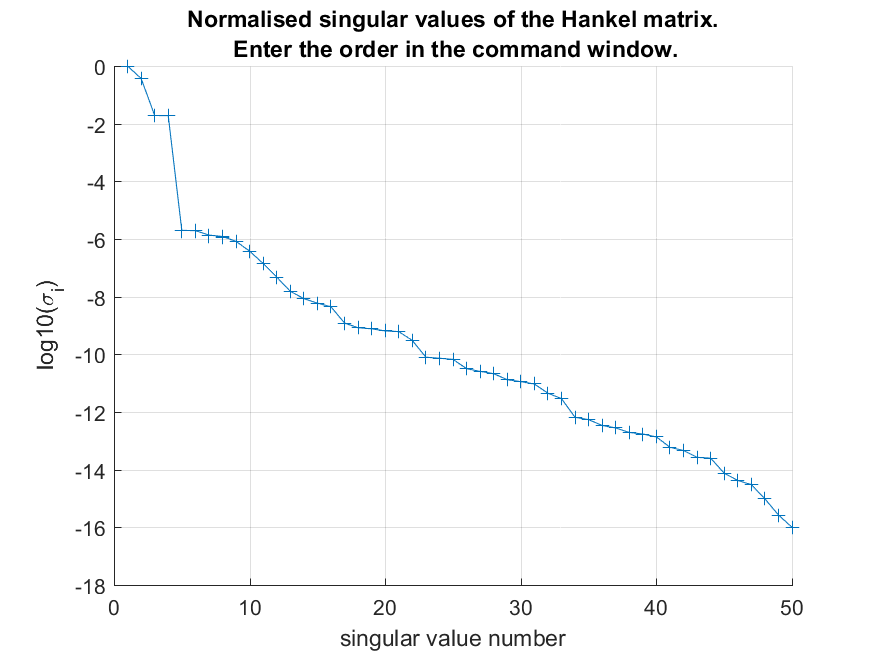
We see that the Hankel matrix has 4 significant singular values. This indicates that there are 4 unstable poles in the system. On the matlab command line, you will see the following message:

Enter the amount of unstable poles:

just type 4 and press enter to confirm the order.

Setting the Hankel size

The default number of Fourier coefficients used to construct the Hankel matrix is 100. This size gives good results for low-order systems. When the amount of unstable poles is large, a larger Hankel matrix is recommmended. You can control the number of Fourier coeffients used in the Hankel matrix as follows:

 poles = PisaEstimate(Z,'numberOfCoefficientsForEstimate',200)

Watch out that you are not asking more coefficients than the amount computed in the projection.

Poles estimated outside disc

During the computation of the system’s poles, there is no guarantee that they are estimated inside of the unit circle. Because we are looking for stable poles, they need to be inside the unit circle by definition, so when the function detects poles estimated outside of the unit circle, it will throw an error:

Error using PisaEstimate (line 158) Estimated a pole outside of the unit circle

When you encounter this error, it has usually one of the following causes:

The order is not chosen correctly. When you ask for an order which is higher than the order of the underlying system, the extra poles will be influenced by the finite interval of the data. This will create poles close to $\theta=\pm \pi / 4$ . Check the singular values of the Hankel matrix and verify whether you are providing the correct order.

The Hankel matrix is too small. For systems with a high amount of poles inside of the unit circle, a larger Hankel matrix is needed. Try increasing the size of the Hankel matrix to resolve the issue with poles estimated outside the circle.

The interpolation error is high. The influence of the interpolation error on the Fourier coefficients can cause issues with the estimated poles. You can check the interpolation error by setting the “EstimateInterpolationError” parameter in PisaProject to true and by plotting the resulting interpolation error. When it is too large, either change a different interpolation mehtod, or increase the amount of samples in the frequency response.

References

A. Cooman, F. Seyfert, and S. Amari, “Estimating unstable poles in simulations of microwave circuits” in 2018 ieee mtt-s international microwave symposium (ims), 2018.