Contents
In this example, we analyse the simulation and measurement of an amplifier designed by Thomas Van den Dries and Indy Magnus as a master student project. The amplifier was built around a BFP520 transistor for operation around 2.5GHz.
First, we determine the stability of the amplifier in simulations, this is a good opportunity to show the unstable part of a stable amplifier. Then, we analyse the measured S-parameters of the amplifier.
We assume here that you are already familiar with how the PisaProject function works. If not, please refer to the pages on closed-loop stability analysis and projection.
Stability analysis in simulation
The following simulation set-up was used in ADS to perform a closed-loop stability analysis:
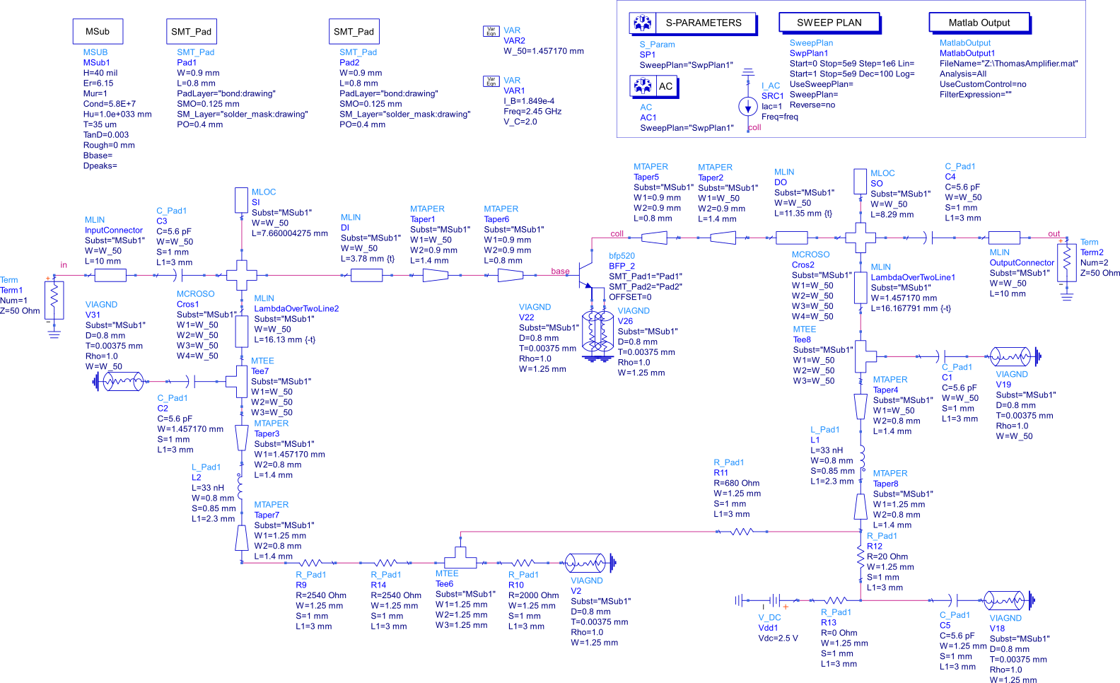
We run two simulations on this setup. An AC simulation in which we perturb the collector with an AC current source and measure the voltage response at the collector, base, input and output of the circuit. The second simulation we run in an S-parameter simulation.
Both simulations are run on the same frequency grid, which is a combination of a logarithmic frequency grid (which will nicely capture the low-frequency dynamics of the circuit) and a linear frequency grid (to have enough points in the high-frequency range).
We load the simulation results using the ADSimportSimData function
simres = ADSimportSimData('.\data\MeasuredAmplifier.mat'); |
simres is now a matlab struct with two fields:
- sim1_AC, which contains the AC simulation results
- sim2_S, which contains the S-parameter simulation results.
We want to analyse the circuit impedance to determine its stability. Therefore, we combine the four voltage responses of the circuit in an impedance vector.
freq = simres.sim1_AC.freq data = zeros(4,1,length(freq)); data(1,1,:) = simdata.sim2_AC.base; data(2,1,:) = simdata.sim2_AC.coll; data(3,1,:) = simdata.sim2_AC.in; data(4,1,:) = simdata.sim2_AC.out; |
with this data, we create an FRM object.
Z = FRM(data,'Freq',freq,'normalisation',LowpassNormalisation(freq)); |
Because we know the impedance function very close to DC, we can use a lowpass normalisation in this stability analysis. This will change once we analyse the measured data. We then call the PisaProject function to perform the projection. Because the data is noiseless, we can use a rational approximation method to obtain the highest accuracy:
PROJ = PisaProject(Z,'Interpolation',RationalInterpolation); |
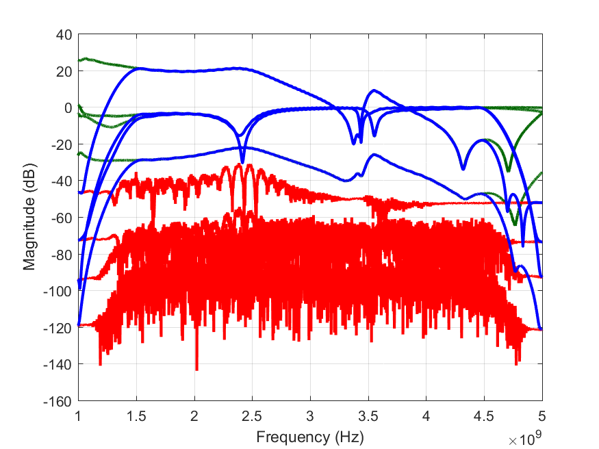
We then plot the original data and its stable and unstable parts. The result is the following:
figure plot( Z ,'Color',[0 0.4 0],'linewidth',2) plot(PROJ.stable ,'Color','b','linewidth',2) plot(PROJ.unstable,'Color','r','linewidth',2) xlim([0 max(Z.Freq)]); ylim([-120 60]); |

This shows a very low unstable part, so we can conclude that the circuit is stable.
Stability analysis of the measurements
This amplifier was built and its response was measured using a vector network analyser. We know that the amplifier is stable (it did not oscillate during measurements), but we want to show how the projection method performs on noisy data.
The measurements were saved as an s2p file. Pisa includes a parser for touchstone files, so we use that parser to load the measured S-parameters into matlab. Because we are working with measurements of a multiport circuit, we create a MultiPort object, which inherits from FRM. We use the read function from the Multiport class to load the measurement data:
Smeasured = MultiPort.read(fullfile('.','data','MeasuredAmplifier.s2p')); |
We will now determine whether the S-parameters of the measured circuit are stable. Note that this is different from analysing the impedance presented by the circuit as we did on the simulation result, because that impedance depends on the load impedance connected to the circuit, while the S-parameters don’t.
The PisaProject also accepts MultiPort objects as inputs, so we just pass Smeasured to PisaProject. We don’t know the S-parameters at low frequencies, as the VNA cannot measure at DC, so we use a bandpass normalisation in the analysis. The default normalisation for MultiPort objects is bandpass, so we have nothing to change.
Because the data is noisy, it is a bad idea to use rational interpolation, as it enforces a continuous first derivative. We use Linear interpolation instead, which is the best we can do on noisy data.
PROJmeasured = PisaProject(Smeasured,'Interpolation',LinearInterpolation); |
We plot the result of the analysis:
figure plot(Smeasured,'Color',[0 0.4 0]); plot(PROJmeasured.unstable,'Color','r'); plot(PROJmeasured.stable ,'Color','b'); xlim([min(Smeasured.Freq) max(Smeasured.Freq)]) |
In the result, we notice that the unstable part is very noisy. Around 2.5GHz, some calibration artefacts are visible in the unstable part as well
Download code and workspace
Click here to download the ADS workspace with all the examples and the matlab code to run pisa.